Created by Volha Kaskevich, this practical online Academy teaches GIS, remote sensing and Earth Observation through real environmental data—from scientific Python and geospatial analysis to Google Earth Engine and machine learning.
Investigate the August 2021 northern Evia wildfire with an authoritative Copernicus perimeter, harmonized Sentinel-2 imagery, continuous dNBR and matched-season recovery trajectories. Measure spectral recovery without confusing it with ecological recovery.
01
Prepare the data
Select, filter, mask, and align six years of surface reflectance.
02
Measure the change
Compare burn severity and vegetation recovery over time.
03
Explain the result
Check uncertainty and present a short, clear scientific briefing.
All 53 lessons, twelve chapter practica and the final UAV and Satellite Analysis Pipeline capstone are available. The pathway progresses from spatial foundations through advanced image analysis and production geospatial computing, with one reviewable portfolio artifact at every chapter boundary.
Module 3 overview
Remote Sensing Modelling
Turn remote-sensing observations into defensible predictions by making the scientific claim, training evidence, validation design, uncertainty and operational domain explicit.
Final project
Environmental Monitoring Project
Prerequisites
Modules 1–2 or equivalent competence in scientific Python, tabular data, spatial support, raster and EO products, spatial sampling, model QA and reproducible delivery
01Question
02Target and unit
03Predictor hypotheses
04Training evidence
05Baseline and model
06Independent validation
07Uncertainty and applicability
08Operational monitoring
Module outcomes
By the end of the module, you can:
Formulate predictive EO questions without confusing association, explanation and causality
Define target, prediction unit, domain and operational predictor contract
Establish baselines and train reproducible tree-ensemble and XGBoost models
Design spatial, temporal and nested validation that matches the intended claim
Evaluate regression, classification, calibration and structured failure
Map domain of applicability and prediction uncertainty
Operationalise bounded local and Earth Engine modelling workflows
All thirty lessons and the independently assessed Environmental Monitoring Project capstone are available. The capstone integrates the complete predictive evidence chain into one professional handover.
1.1WEEKS 01Lesson 1.1CurrentWelcome to Scientific ProgrammingUnderstand scientific programming, learn how a notebook works, run your first Python instructions and preserve the first Vegetation Data Explorer checkpoint.Jupyter NotebookPythonBaltic coastal meadow studyClose lesson
Lesson 1.1 of 12CoreBeginner60–75 minutes0 of 5 checks completed
You already know how scientists ask questions, distinguish observations from interpretations and judge whether evidence is relevant. You do not need programming knowledge. Your scientific experience is the starting point.
In this lesson
You will turn one ecological question into a small, inspectable notebook record. You will learn what programming and scientific programming mean, how Jupyter, a notebook file, Python and the kernel divide their roles, how the computer executes an instruction and how to preserve the result for another person to inspect.
Why this comes now
Every later table, map, raster and model depends on instructions being executed in a known order and on the scientist separating computational success from scientific validity. Learning that distinction before variables or datasets prevents code from becoming an unexplained sequence of commands.
You will use this later
Lesson 2 adds scientific values to the notebook. Lesson 6 develops systematic debugging. Lesson 8 introduces the published Baltic coastal-meadow table. Every later Academy project uses the same question → instruction → output → validation → interpretation cycle.
1. Scientific question and computational method
Learning outcome
By the end of this lesson, you can explain scientific programming; distinguish a scientific question from a computational instruction; explain the roles of Jupyter, a notebook file, Python and the kernel; distinguish Markdown and code cells; run simple instructions in order; predict output before execution; recognise and repair a simple SyntaxError; restart and clean-run a notebook; preserve it for inspection; and explain why successful execution does not prove scientific validity.
Prerequisites: None. You do not need to know Python, files, folders, terminals or notebooks.
Why this matters
Core lesson How does a scientific question become something a computer can actually execute?
You have joined a research group studying Baltic coastal meadows. Across the module, your working question is:
How can field measurements help us describe and compare vegetation patterns across Baltic coastal meadow plots?
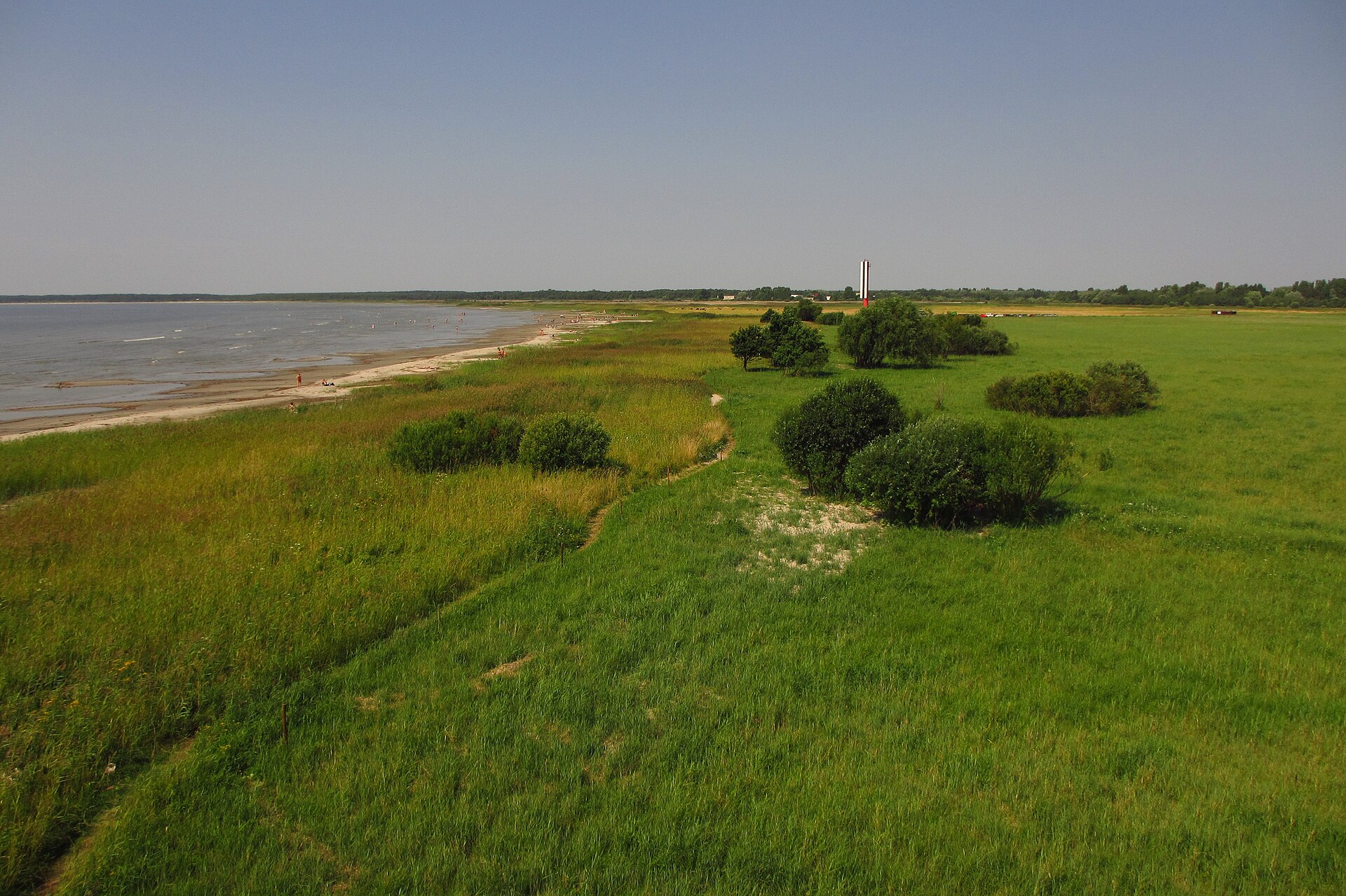
Pärnu coastal meadow, Estonia — what observations and metadata would be needed to turn this landscape into scientific data?
Scientific context, not lesson data. Photograph by Marko Vainu, 7 August 2013, Wikimedia Commons, CC BY-SA 4.0. The photograph is not part of the published Baltic coastal plant-traits dataset and no values are inferred from it here.
Before thinking about code, inspect the landscape. What would need to be defined before a computer could compare its vegetation: the observation unit, field protocol, dates, locations, measurements, quality checks, or something else? The computer cannot choose these scientific meanings for you.
A scientific question is not yet a computational method. To analyse it, a scientist must turn decisions into instructions: which data to inspect, which values to compare, what to calculate and how to check the result.
Programming means writing instructions a computer can execute. Scientific programming means using explicit, repeatable computer instructions to investigate scientific evidence while keeping scientific judgement with the researcher.
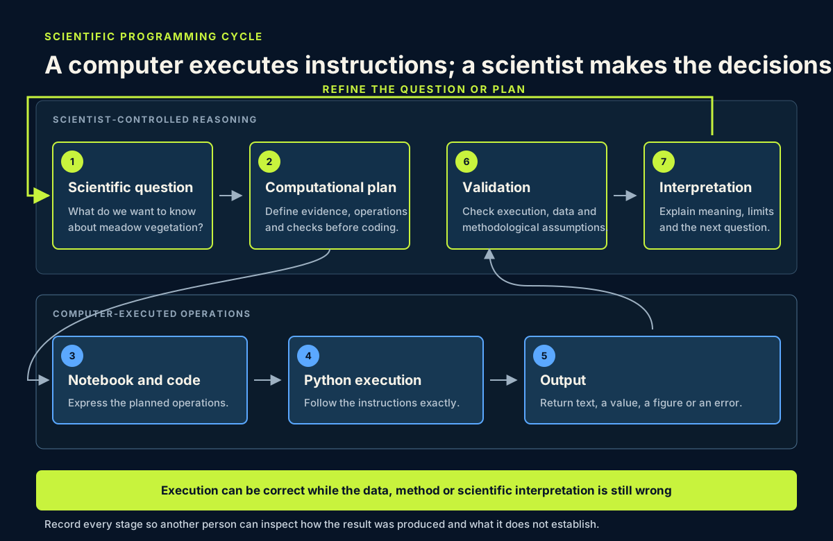
The relationship is a cycle:
The scientist asks a question.
An analysis plan defines operations and checks.
Notebook code expresses exact instructions.
Python executes those instructions.
The notebook records output, including errors.
The scientist validates execution, data and method.
The scientist interprets what the output means and does not mean.
The evidence may lead back to a revised question or plan.
Scientific programming cycle — reasoning controls the computation and returns to the question
The arrows are not a guarantee of correctness. They make the reasoning inspectable. Code can execute exactly as written even when the wrong evidence was selected or the scientific question was translated badly.
Core lesson Write your own one-sentence definition of scientific programming in your private notes. Include both repeatable instructions and scientific judgement.
Learner action
Write one scientific question about Baltic coastal meadow vegetation that could eventually be investigated using field measurements and Earth Observation data. Do not try to write code yet.
2. Meet the notebook
A file is a saved digital item with a name. A Jupyter notebook is a file ending in .ipynb. It can keep the question, code, output and interpretation together, which makes the route from evidence to conclusion easier to inspect than a final Word report alone.
A notebook contains cells:
A Markdown cell holds headings, explanations, predictions and interpretations. Running it formats the text.
A code cell holds Python instructions. Running it sends those instructions to Python and returns output or an error.
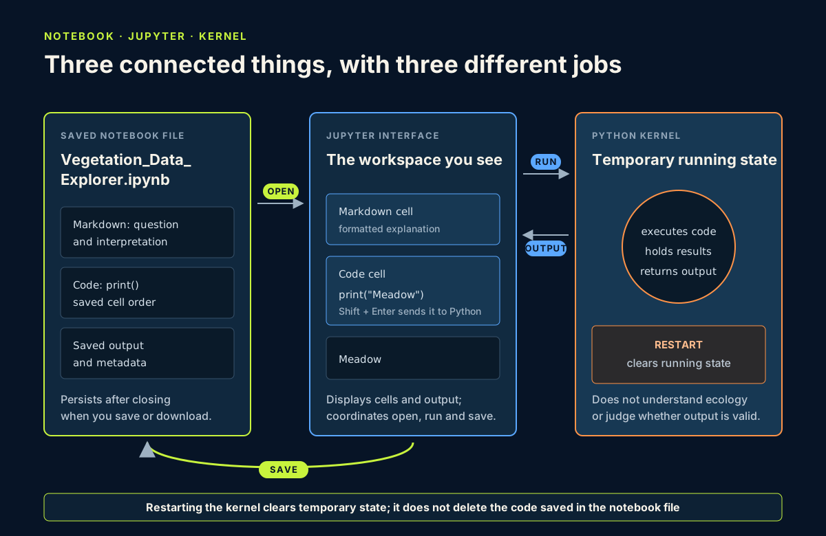
Four names that beginners often mix up
Notebook file: the saved .ipynb record containing cells, saved output and metadata.
Jupyter: the interface that opens the file, displays cells and sends code to be run.
Python: the programming language used to express the instructions.
Kernel: the running Python process that executes code and temporarily remembers the current computational state.
Notebook, Jupyter and kernel mental model — restarting clears temporary state but does not delete saved code
When you choose Save, Jupyter updates the notebook file. When you choose Restart Kernel, Jupyter clears the kernel's temporary running state. Your saved code remains in the notebook. When you choose Run All, Jupyter sends code cells to a fresh kernel in notebook order. These actions are related, but they are not interchangeable.
Choose the right scientific record
Different formats support different parts of professional work:
Format
Best used for
Important limitation
Word or similar document
Polished narrative, review and final reporting
The calculation that produced a result is usually separate
Jupyter notebook
Developing an analysis while keeping question, code, output and interpretation together
Cells can be run out of order and hidden state can make a result difficult to reproduce
Python script
Repeatable processing that should run from beginning to end
Narrative and exploratory output require deliberate documentation
The notebook is the right first instrument because it keeps beginner explanation beside executable evidence. It is not automatically superior to the alternatives. A mature project often uses notebooks for investigation, scripts for stable processing and a report for communication.
The kernel is the running Python process behind the notebook. When you run a code cell, Jupyter sends the cell to the kernel. The kernel reads instructions from top to bottom within that cell and stops if it reaches an instruction it cannot complete.
The kernel also preserves the consequences of cells you already ran until it is restarted. That flexibility helps exploration, but it can hide the order needed to reproduce a result. A professional notebook must therefore pass a clean-run test: restart the kernel, run every required cell from top to bottom and confirm that the result can be regenerated.
Download the starter notebook from the lesson resources below. Keep the downloaded file somewhere you can find again, then rename it exactly:
Vegetation_Data_Explorer.ipynb
Open it in JupyterLab, Jupyter Notebook, or your institution's current Jupyter environment. If you have no installed environment, Try Jupyter provides a browser workspace. Browser workspaces may be temporary, so always download your work before leaving.
Go deeper — why not install everything today? Professional projects often use separate environments and recorded package versions. Those practices matter, but installing and managing environments is not required for this first lesson. The module will introduce reproducibility in stages.
Learner action
Open the starter notebook. Find its title cell, one prediction field and one prepared code cell. Change the learner-name placeholder to your name or researcher identifier, then save.
3. Run the first instruction
The first prepared code cell contains:
print()
Before running it, predict what will appear: the word print, an error, or an empty-looking line. Record the prediction in the Markdown field directly above the code.
Check your understandingBefore you run print(), what output should you predict?
Now select the code cell and press Shift + Enter, or use the Run control.
print is a built-in Python function that sends information to the output area. The parentheses mean “run this function now”. Nothing appears inside the parentheses, so print() produces only a new line. The output looks empty, but Python still completed a valid instruction.
Code walkthrough
print is the function name.
( opens the function call.
There is no value to display.
) closes the call.
The kernel executes the complete instruction and returns a line break.
Learner action
Under the output, add a Markdown sentence explaining why an empty-looking result can still show that an instruction ran.
4. Predict execution order
The next prepared code cell contains three instructions:
print("Vegetation Data Explorer")
print("Study system: Baltic coastal meadows")
print("Question: How does vegetation vary among field plots?")
Predict before running
In the prediction field, write the three lines in the order you expect them to appear. Then run the cell.
Check your understandingA code cell contains three print instructions on three lines. In which order will a fresh kernel execute them?
Expected output:
Vegetation Data Explorer
Study system: Baltic coastal meadows
Question: How does vegetation vary among field plots?
Python works from the first line to the third line. Each print(...) call contains a string: text between straight quotation marks. You will study strings formally in Lesson 2. For now, notice that the quotation marks tell Python where the text begins and ends; they are not shown in the output.
Scientific interpretation
Python displayed a research question, but it did not judge whether the question is answerable, whether the data are suitable or whether the wording is ecologically sound. Execution answers “Did the computer follow the instruction?” Interpretation asks “What does the result mean, and is the method scientifically defensible?”
Scientific note A precise output can still result from weak data, an unsuitable method or an unsupported assumption. Computational correctness and scientific validity must be checked separately.
Diagnose — it worked, but is it scientifically valid?
Imagine that Python displays:
Mean vegetation height = 42.7 cm
Which conclusion is justified?
Vegetation is definitely 42.7 cm high.
Python successfully displayed the supplied or computed value.
Field sampling was scientifically valid.
The measurement represents the entire coastal meadow.
Check your understandingPython displays “Mean vegetation height = 42.7 cm”. Which conclusion is justified by that output alone?
Only the second statement follows from the output. To support the others, you would need evidence about the input values, units, sampling design, calculation, quality control, spatial and temporal scope, and uncertainty. Successful execution is one check in an evidence chain, not the scientific conclusion.
In two sentences, explain the difference between computational success and scientific validity in your notebook.
Learner action
Change only the final printed question so it matches the scientific question you wrote in Block 1. Predict the output order again, run the cell and confirm the lines remain in the expected sequence.
5. Cause and fix one error
Create a new code cell and deliberately type this incomplete instruction:
print("Baltic coastal meadow)
Run it. Python should report a SyntaxError because the opening quotation mark has no matching closing quotation mark. The error is information, not a judgement about your ability.
Check your understandingWhy does print("Baltic coastal meadow) produce a SyntaxError?
When code fails
Read the final error line.
Identify the referenced line.
Compare names and punctuation.
Change one thing.
Run the cell again.
Add the missing straight quotation mark so the corrected cell becomes:
print("Baltic coastal meadow")
Run it again and keep the corrected output. Full debugging and notebook-state management will be taught in Lesson 6.
Common mistake: code in a Markdown cell
If print("Baltic coastal meadow") appears as formatted text instead of producing output, the instruction is probably in a Markdown cell. Change the cell type to Code and run it again.
Learner action
Add a Markdown note below the corrected cell. State what Python reported, which single character was missing and how you knew the fix worked.
6. Save and submit the notebook
Saving updates the notebook in its current workspace. Downloading creates a separate copy that you control. Use both actions:
Confirm the notebook is named Vegetation_Data_Explorer.ipynb.
Save it in Jupyter.
Download a copy to a known folder on your computer.
Reopen the downloaded copy if your environment allows it.
Run the required cells from top to bottom and confirm that the corrected cell succeeds.
Guided practice
Complete the starter notebook's Markdown prompts: project title, researcher name, scientific question, predictions, first execution note and error correction note.
Then complete its handover check:
Restart the kernel.
Use Run All or run every required cell from top to bottom.
Confirm the deliberately broken instruction has been replaced by the corrected version.
Compare the regenerated output with your predictions.
Record whether the notebook passed, and identify any cell that needed correction.
Save and download the clean result.
This is your first QA/QC procedure. It checks execution order and preservation. It does not establish that the scientific question or future data are valid.
Independent challenge
Add one code cell with no more than three print() instructions. Display:
your researcher name or identifier;
one ecological feature you want to understand;
one kind of Earth Observation evidence that might eventually help.
Predict the line order before running. After running, add two Markdown sentences: one identifies the executed instructions and output; the other identifies the scientific judgement that remains yours.
Finish with a professional scenario: imagine a colleague receives only this notebook. Add a Markdown note titled ### Handover note that tells them the question, which cells to run, what successful output looks like and what the output does not prove. Do not explain Python generally; explain how to inspect this specific scientific record.
Independent handover test
Close the notebook, reopen the downloaded copy and use only the visible instructions in the file. If you cannot reproduce the output without remembering an undocumented step, revise the notebook and repeat the test.
Learner action
Use the submission checklist shown below the lesson. Upload the renamed notebook and one screenshot, then add the requested written explanation in the submission panel.
7. Reflection and summary
Close the notes — 3-minute recall
Close or cover the lesson text. Without running code, answer from memory:
What is scientific programming?
When would you use a Markdown cell rather than a code cell?
What does the kernel do?
Why restart the kernel and run the notebook from top to bottom?
Why does successful code execution not prove a scientific conclusion?
Then reopen the lesson, check your answers and correct only what you could not explain accurately.
Check your understandingWhat is the strongest reason to restart the kernel and run all required cells from top to bottom?
Reflection
Write short answers in your private notes:
What is scientific programming, in one sentence?
When should you use a Markdown cell, and when should you use a code cell?
What did the kernel do when it reached the incomplete string?
Why does a successfully executed cell not prove that a scientific claim is valid?
Where is your downloaded notebook stored?
When would a script or a report be a better format than a notebook?
Portfolio artifact
Artifact 01 — Scientific Notebook Foundation
Your Vegetation_Data_Explorer.ipynb now contains a project title, a researcher identifier, a scientific question, predictions, executable Python instructions, a corrected SyntaxError, an interpretation, a clean-run QA record, a handover note and a reflection on scientific interpretation. It is the first checkpoint in Portfolio Project 1 — Vegetation Data Explorer, not a separate mini-project. Keep this notebook: Lesson 2 extends it rather than replacing it.
Summary
You can now describe scientific programming as a partnership between explicit computation and scientific judgement. You can choose why a notebook is appropriate, use its two essential cell types, run simple instructions in order, correct one syntax error and preserve a clean, inspectable record. Lesson 2 will add scientific values and names without discarding this foundation.
The example is already entered. Change it when the lesson asks you to experiment, then select Run Python.
Python runs privately on this device
Output
Run the code to see its output here.
Standard Python and supported scientific packages run here without an account. Examples that depend on lesson files can still be developed here, then completed in the downloadable notebook with those files.
Current lesson
Submission guide
Checklist and review rubric
Before submitting
The starter notebook is renamed Vegetation_Data_Explorer.ipynb
All required Markdown and code cells are present and executed
The deliberately broken print instruction is corrected
A clean restart-and-Run-All check is recorded
The notebook is saved, reopened and a downloaded copy is retained
The handover note identifies the question, run sequence, expected output and interpretation limit
The written answer distinguishes code cells from Markdown cells
The reflection is complete
Review dimensions
Technical correctness
Required cells run and the simple syntax error is corrected
Conceptual understanding
Explains scientific programming and code versus Markdown
Reproducibility
Notebook is clearly named, clean-run from top to bottom, reopened and preserved
Scientific communication
Handover note separates successful execution from scientific interpretation
Review statuses
Not submitted
Submitted
Revision requested
Meets expectations
Portfolio ready
Program task
Portfolio checkpoint 01 · Environment notebook
Upload Vegetation_Data_Explorer.ipynb and a screenshot that shows the notebook title, a code cell and its output. In the written result field, explain in 120–180 words what scientific programming is and why execution is different from scientific interpretation. Before uploading, restart the kernel and run all cells from top to bottom.
Learner submission · browser prototypeMap, imagery, and interpretation
Up to 5 files · 50 MB each
Learner submission prototype: private and saved only in this browser. Sign in to synchronize it and contact an instructor.
Private learner–instructor conversationQuestions, revision requests, and feedback
Sign in to share private comments with an instructor.
Shared lesson discussion
Sign in to read or join the optional discussion for this lesson.
Technical and source information
Tested Python
Python 3.12.3
Tested Jupyter environment
JupyterLab 4 / Notebook 7 compatible notebook format (nbformat 4.5)
Last technical review
25 August 2026
Portfolio artifact
Scientific Notebook Foundation
Prerequisites
None
Dataset citation
Baltic coastal plant traits 2024, Zenodo record 20083250, https://doi.org/10.5281/zenodo.20083250
Official documentation · Definition of the first Python function used in this lesson.
1.2WEEKS 02Lesson 1.2Variables and Scientific DataRepresent scientific values with clear variable names and appropriate strings, numbers, Booleans and missing values without confusing type with validity.PythonScientific valuesSALS1 field observationOpen lesson1.3WEEKS 03Lesson 1.3Collections for Ecological InformationUse lists for editable species observations and dictionaries for named plot fields, with brief supporting uses for tuples and sets.Python collectionsVegetation metadataCoordinate conventionsOpen lesson1.4WEEKS 04Lesson 1.4Conditions and Data-Quality RulesTranslate transparent scientific criteria into auditable Python decisions while preserving missing values and source measurements.Python conditionsQuality flagsMissing-value reasoningOpen lesson1.5WEEKS 05Lesson 1.5Repetition, Loops and Vectorised ThinkingApply one verified method consistently across several plot records and prepare to reason about whole numerical collections.Python loopsAccumulatorsHand verificationOpen lesson1.6WEEKS 06Lesson 1.6Functions, Errors and DebuggingTurn scientific rules into tested reusable functions and diagnose failures from tracebacks and controlled evidence.Python functionsTest casesDebugging workflowOpen lesson1.7WEEKS 07Lesson 1.7NumPy and Numerical ArraysRepresent verified ecological sequences as numerical arrays, inspect shape and dtype, and apply aligned vectorised masks.NumPyBoolean masksPublished richness valuesOpen lesson1.8WEEKS 08Lesson 1.8Open the Published Dataset with pandasLoad the complete Zenodo CSV through a reproducible project path and verify its structure before analysis.pandasPathlibZenodo datasetOpen lesson1.9WEEKS 09Lesson 1.9Missing Values, Types and Data QualityProfile real missingness and data types, apply field-specific checks and preserve every decision in an audit trail.pandas quality profileMissingnessDecision logOpen lesson1.10WEEKS 10Lesson 1.10Filter, Group and SummariseDefine a countable analysis population and produce grouped summaries that retain sample size, centre, spread and limitations.pandas filteringGroupByDescriptive statisticsOpen lesson1.11WEEKS 11Lesson 1.11Join, Reshape and VisualiseJoin summaries with validated keys, expose unsampled combinations and communicate one comparison in a clear scientific figure.pandas mergePivot tablesMatplotlibOpen lesson1.12WEEKS 12Lesson 1.12Vegetation Data Explorer ProjectAssemble the complete notebook into a reproducible claim–evidence chain and deliver a defensible ecological briefing.Reproducible notebookScientific figuresPortfolio briefingOpen lesson
2.1CHAPTER 1Lesson 2.1What Makes Data Geospatial?Distinguish ordinary tables, vector features, raster grids and spatial data with incomplete reference metadata.Spatial reasoningVectorRasterOpen lesson2.2CHAPTER 1Lesson 2.2Coordinate Reference SystemsChoose, inspect, assign and transform coordinate reference systems without confusing metadata repair with reprojection.pyprojGeoPandasEPSGOpen lesson2.3CHAPTER 1Lesson 2.3Scale, Resolution and Spatial SupportRelate field quadrats, UAV pixels and satellite pixels to the ecological processes they can validly represent.ScaleResolutionSpatial supportOpen lesson2.4CHAPTER 1Lesson 2.4Geospatial Formats and MetadataSelect formats that preserve geometry, grids, metadata and efficient access across local and cloud workflows.GeoPackageGeoParquetCOGZarrOpen lessonPRACTICUMCHAPTER 1Chapter practicumAccept, Review or Reject?Make a documented data-acceptance decision from incomplete spatial evidence before analysis begins.Evidence reviewRisk classificationDecision recordOpen lesson2.5CHAPTER 2Lesson 2.5GeoPandas and Spatial TablesExtend pandas reasoning to geometry, CRS, spatial bounds and geospatial file exchange.GeoPandasGeoPackageGeoJSONOpen lesson2.6CHAPTER 2Lesson 2.6Geometry with ShapelyConstruct and evaluate geometry operations while separating computational validity from ecological justification.ShapelyGeometryPredicatesOpen lesson2.7CHAPTER 2Lesson 2.7Spatial Joins, Overlay and Nearest NeighboursMatch features through spatial relationships while auditing duplicates, unmatched records and one-to-many results.sjoinoverlaynearestOpen lesson2.8CHAPTER 2Lesson 2.8Spatial Indexing and PerformanceUnderstand how bounding-box indexes reduce candidate comparisons without changing spatial predicates.Spatial indexSTRtreeProfilingOpen lesson2.9CHAPTER 2Lesson 2.9Topology, Geometry Cleaning and Data IntegrityClean multipart, invalid and duplicated geometries while retaining an explicit topology decision log.DissolveExplodeTopology QAOpen lesson2.10CHAPTER 2Lesson 2.10QGIS for Professional Spatial QAUse QGIS as a visual verification companion to reproducible Python processing.QGISVisual QAMap exportOpen lessonPRACTICUMCHAPTER 2Chapter practicumVector Handover ReviewAudit a vector delivery as if you were accepting responsibility for the next professional analysis stage.Vector QAReconciliationHandover decisionOpen lesson2.11CHAPTER 3Lesson 2.11What Is a Raster Really?Build a rigorous mental model of values, grids, spatial reference, valid support and measurement semantics before processing.Raster modelAffine transformNoDataOpen lesson2.12CHAPTER 3Lesson 2.12Rasterio: Read, Inspect and Write Spatial GridsInspect a GeoTIFF spatial contract, read masked values and verify a written derivative through a complete round trip.RasterioNumPyRound-trip QAOpen lesson2.13CHAPTER 3Lesson 2.13Crop, Mask, Reproject and ResampleSeparate four transformations and choose their sequence and resampling logic from scientific meaning.RasterioResamplingMaskingOpen lesson2.14CHAPTER 3Lesson 2.14Raster Alignment and Grid IntegrityDetect grid mismatch, design a common lattice and prove cell-by-cell compatibility explicitly.Grid alignmentTarget gridQA functionOpen lesson2.15CHAPTER 3Lesson 2.15Raster–Vector IntegrationExtract raster evidence to vector sampling units through a spatial-support decision rather than a default pixel lookup.SamplingZonal statisticsSpatial supportOpen lesson2.16CHAPTER 3Lesson 2.16Large Raster ProcessingEstimate memory, process stored blocks and use virtual transformed views without changing numerical meaning.WindowsBlocksWarpedVRTOpen lesson2.17CHAPTER 3Lesson 2.17Terrain Analysis with DEM and DSMInterpret elevation surfaces and derive slope, aspect and hillshade without losing vertical-reference and surface meaning.DEM / DSM / DTMSlope and aspectTerrain QAOpen lessonPRACTICUMCHAPTER 3Chapter practicumBuild an Analysis-Ready Raster StackHarmonise five deliberately different raster inputs into one validated grid with extraction and QA evidence.Raster harmonisationAlignment QAProfessional handoverOpen lesson2.18CHAPTER 4Lesson 2.18UAV Remote Sensing FundamentalsTreat a UAV as a complete observing system and distinguish direct sensor records from derived geospatial products.UAV systemsSensor typesProduct provenanceOpen lesson2.19CHAPTER 4Lesson 2.19Mission Design: Altitude, GSD and OverlapCalculate nominal sampling geometry and evaluate how altitude, footprint, overlap, speed, shutter and terrain interact.Mission geometryGSDOverlapOpen lesson2.20CHAPTER 4Lesson 2.20Sensors, Illumination and Radiometric QualityTrace digital values through exposure, illumination and calibration evidence before calling them comparable reflectance.RadiometryCalibrationBand registrationOpen lesson2.21CHAPTER 4Lesson 2.21Georeferencing: GNSS, GCP, RTK and PPKSeparate positioning constraints from independent validation and diagnose horizontal, vertical and local error.GNSSControl pointsAccuracy QAOpen lesson2.22CHAPTER 4Lesson 2.22Structure from Motion and Photogrammetric ReconstructionTrace overlapping perspective images through a software-independent three-dimensional reconstruction workflow.Structure from MotionBundle adjustmentDense reconstructionOpen lesson2.23CHAPTER 4Lesson 2.23Point Clouds, DSM, DTM and OrthomosaicsInterpret common UAV products from the observations and models that created them.Point cloudsSurface modelsOrthomosaicsOpen lesson2.24CHAPTER 4Lesson 2.24UAV Product QA and Error DiagnosisIntegrate mission, image, photogrammetry, georeferencing, mosaic, surface, multispectral and temporal evidence.UAV QAError diagnosisDecision matrixOpen lesson2.25CHAPTER 4Lesson 2.25UAV Multispectral Processing PipelineBuild an accepted multispectral subset with explicit radiometric, geometric, mask and provenance gates.Multispectral stackSafe indicesRaster extractionOpen lessonPRACTICUMCHAPTER 4Chapter practicumEvaluate a UAV Survey Before Scientific AnalysisAudit a deliberately imperfect UAV handover and decide which products and regions are defensible for ecological use.UAV product QAPhotogrammetry evidenceProfessional handoverOpen lesson2.26CHAPTER 5Lesson 2.26Optical Remote SensingConnect electromagnetic interactions, sensor bands and product levels to interpretable surface reflectance.Sentinel-2LandsatReflectanceOpen lesson2.27CHAPTER 5Lesson 2.27Vegetation and Spectral IndicesUse vegetation indices as sensor- and context-dependent proxies rather than direct ecological measurements.NDVIRed edgeSAVIOpen lesson2.28CHAPTER 5Lesson 2.28SAR FundamentalsInterpret Sentinel-1 backscatter through acquisition geometry, surface properties and preprocessing choices.Sentinel-1VV/VHBackscatterOpen lesson2.29CHAPTER 5Lesson 2.29Hyperspectral Remote SensingRecognise when dense narrow-band measurements provide useful spectral evidence and additional preprocessing burden.HyperspectralSpectral curvesSNROpen lesson2.30CHAPTER 5Lesson 2.30LiDAR and Point CloudsTurn discrete three-dimensional returns into terrain and vegetation-structure products.LiDARPoint cloudsCanopy heightOpen lessonPRACTICUMCHAPTER 5Chapter practicumBuild a Defensible Satellite Evidence PackageIntegrate optical, spectral-index, SAR, imaging-spectroscopy and LiDAR evidence without forcing incompatible measurements into one claim.Cross-sensor QAEvidence integrationScientific decisionOpen lesson2.31CHAPTER 6Lesson 2.31Spatial AutocorrelationRecognise spatial dependence and its consequences for inference and validation.Moran's IWeightsSpatial dependenceOpen lesson2.32CHAPTER 6Lesson 2.32Spatial Sampling and BiasDesign and diagnose sampling that represents spatial heterogeneity without hidden clustering.Sampling designBiasStratificationOpen lesson2.33CHAPTER 6Lesson 2.33Interpolation and GeostatisticsTreat interpolation as a model of spatial continuity with assumptions and prediction uncertainty.IDWVariogramKrigingOpen lesson2.34CHAPTER 6Lesson 2.34Spatial Regression ConceptsRecognise when ordinary regression residuals violate independence and what spatial models attempt to address.Spatial lagSpatial errorGWROpen lessonPRACTICUMCHAPTER 6Chapter practicumDesign and Defend a Spatial Inference PlanAudit sampling, spatial dependence, interpolation and regression as one geographically validated evidence system.Spatial inferenceGeographic validationRelease decisionOpen lesson2.35CHAPTER 7Lesson 2.35SQL for Geospatial ScientistsQuery environmental tables with explicit filtering, grouping and relational joins.SQLJOINGROUP BYOpen lesson2.36CHAPTER 7Lesson 2.36PostGIS FundamentalsMove vector relationships from in-memory Python to indexed database queries.PostGISSRIDSpatial SQLOpen lesson2.37CHAPTER 7Lesson 2.37Managing Large Spatial DataChoose when files, columnar objects or a spatial database best support scale and collaboration.GeoParquetPostGISObject storageOpen lessonPRACTICUMCHAPTER 7Chapter practicumBuild a Governed Spatial Database HandoverConvert an imperfect spatial-data handover into a controlled relational, spatial and storage architecture with traceable release evidence.Relational integritySpatial SQLData governanceOpen lesson2.38CHAPTER 8Lesson 2.38Xarray and RioxarrayWork with labelled multidimensional arrays that preserve coordinates, dimensions and attributes.XarrayRioxarrayLabelled arraysOpen lesson2.39CHAPTER 8Lesson 2.39EO Data CubesExtend one spatial band into band and time dimensions while preserving comparable observations.Data cubeTime seriesMaskingOpen lesson2.40CHAPTER 8Lesson 2.40Dask and Lazy ComputationPlan chunked computations that fit memory without turning the lesson into distributed-systems engineering.DaskChunksLazy executionOpen lesson2.41CHAPTER 8Lesson 2.41COG, Zarr and Cloud-Native FormatsMatch tiled range-readable rasters and chunked arrays to remote access patterns.COGZarrRange requestsOpen lesson2.42CHAPTER 8Lesson 2.42STACDiscover cloud-hosted Earth Observation assets through consistent catalog metadata.STACCatalogSearchOpen lessonPRACTICUMCHAPTER 8Chapter practicumBuild a Reproducible Cloud-Native EO Evidence CubeConnect STAC discovery, labelled cube eligibility, bounded Dask execution and validated COG/Zarr publication in one traceable scientific package.Xarray and DaskCOG and ZarrSTAC provenanceOpen lesson2.43CHAPTER 9Lesson 2.43Web Maps and Spatial ServicesUnderstand how browsers request tiles, features and coverages from spatial services.XYZWMS/WFSVector tilesOpen lesson2.44CHAPTER 9Lesson 2.44Interactive MappingCommunicate spatial results through a focused interactive map without teaching full frontend engineering.FoliumMapLibreAccessibilityOpen lesson2.45CHAPTER 9Lesson 2.45OGC Standards and InteroperabilityRelate established web services, OGC APIs, COG and STAC across professional systems.OGC APIInteroperabilityServicesOpen lessonPRACTICUMCHAPTER 9Chapter practicumDeliver an Accessible Environmental Monitoring MapTurn reviewed EO evidence into a purpose-led public map, equivalent table and tested interoperable handover without exposing restricted information.Web delivery architectureAccessible interactive mappingOGC interoperabilityOpen lesson2.46CHAPTER 10Lesson 2.46ArcGIS Professional EcosystemPosition ArcGIS components within a broader interoperable geospatial architecture.ArcGIS ProEnterpriseInteroperabilityOpen lessonPRACTICUMCHAPTER 10Chapter practicumDesign a Portable Coastal-Meadow GIS ArchitectureAllocate ArcGIS and open components by role, prove cross-ecosystem equivalence, and defend a governed architecture with an exit path.Enterprise architectureWorkflow translationMigration evidenceOpen lesson2.47CHAPTER 11Lesson 2.47Image Segmentation FundamentalsSeparate pixels into meaningful regions before classification or measurement.SegmentationTextureObjectsOpen lesson2.48CHAPTER 11Lesson 2.48Deep Learning for Geospatial ImagesUnderstand the image-to-patch-to-probability-to-mask workflow before using model APIs.CNNU-NetSemantic segmentationOpen lesson2.49CHAPTER 11Lesson 2.49Geospatial Deep Learning QAAudit leakage, domain shift, annotation uncertainty and false confidence in mapped predictions.Spatial leakageDomain shiftCalibrationOpen lessonPRACTICUMCHAPTER 11Chapter practicumAudit a Meadow Segmentation ProductDesign, test and communicate an image-segmentation workflow whose labels, spatial splits, thresholds and failure geography are fit for ecological use.Object-based analysisSpatial validationModel QAOpen lesson2.50CHAPTER 12Lesson 2.50APIs and Automated Data AcquisitionRetrieve versioned environmental data robustly while respecting authentication, pagination and rate limits.HTTPJSONRetriesOpen lesson2.51CHAPTER 12Lesson 2.51Command-Line Geospatial ToolsUse inspection, conversion and warping commands as composable professional operations.GDALogr2ogrrioOpen lesson2.52CHAPTER 12Lesson 2.52Docker for Geospatial ReproducibilityPackage difficult native dependencies and project commands into a repeatable execution environment.DockerGDALEnvironmentOpen lesson2.53CHAPTER 12Lesson 2.53Workflow Automation and CITurn the complete pipeline into validated stages that run consistently on every change.GitHub ActionsTestsArtifactsOpen lessonPRACTICUMCHAPTER 12Chapter practicumProductionise the Coastal-Meadow PipelineTurn a reviewed analysis into a versioned, containerised and continuously tested workflow with recoverable acquisition and release evidence.API acquisitionContainersContinuous integrationOpen lessonCapstoneCAPSTONECapstoneUAV and Satellite Analysis PipelineIntegrate field plots, vector zones, UAV products, satellite observations and production QA into one defensible professional delivery.Pipeline designSpatial validationProfessional deliveryOpen lesson
3.1CHAPTER 1Lesson 3.1Prediction, Inference and ExplanationSeparate predictive claims from description, explanation and causal inference before selecting an algorithm.Scientific reasoningPrediction contractClaim boundariesOpen lesson3.2CHAPTER 1Lesson 3.2Define the Target and Prediction UnitSpecify exactly what is predicted, how it was observed, and what receives one prediction.Target contractSpatial supportPrediction domainOpen lesson3.3CHAPTER 1Lesson 3.3Design Predictors and Modelling HypothesesChoose operationally available predictors through measurement reasoning rather than correlation hunting.Predictor hypothesesTraining-serving skewProxiesOpen lesson3.4CHAPTER 1Lesson 3.4Build the Modelling Dataset and Pre-register the ExperimentCreate one auditable row per modelling observation and freeze the evaluation contract before fitting.Data contractFold registryExperiment planOpen lesson3.5CHAPTER 2Lesson 3.5What Does a Useful Model Need to Beat?Define naive and simple baselines before judging complexity.BaselinesModel skillBias–varianceOpen lesson3.6CHAPTER 2Lesson 3.6Trees, Ensembles and BoostingReason from decision-tree partitions to bagging and sequential error correction.Decision treesRandom ForestGradient boostingOpen lesson3.7CHAPTER 2Lesson 3.7XGBoost from First PrinciplesConnect loss, additive trees, regularisation and learning rate to model behaviour.XGBoostObjectivesRegularisationOpen lesson3.8CHAPTER 2Lesson 3.8Train the First Defensible XGBoost ModelFit an untuned, reproducible candidate against a declared baseline and folds.XGBRegressorMetadataSerializationOpen lesson3.9CHAPTER 3Lesson 3.9Validation Is Part of the ModelTreat the withheld evidence and its destination claim as part of the scientific model.GeneralisationCross-validationProximity leakageOpen lesson3.10CHAPTER 3Lesson 3.10Spatial, Grouped and Leave-Location-Out ValidationMatch row, group, block, site and buffered folds to the intended spatial transfer claim.GroupKFoldSpatial blocksLeaveOneGroupOutOpen lesson3.11CHAPTER 3Lesson 3.11Temporal and Spatiotemporal ValidationEvaluate future and future-site transfer without allowing later evidence to move backward in time.Temporal holdoutRolling originDriftOpen lesson3.12CHAPTER 3Lesson 3.12Nested Model Selection and Leakage PreventionKeep inner procedure selection inside outer generalisation assessment and audit every leakage route.Nested CVPipelineLeakage auditOpen lesson3.13CHAPTER 4Lesson 3.13Hyperparameter OptimisationDesign a bounded, reproducible search inside nested development evidence and compare it fairly with the untuned candidate.RandomizedSearchCVGrouped inner foldsSearch protocolOpen lesson3.14CHAPTER 4Lesson 3.14Early Stopping, Regularisation and Learning DynamicsRead training and structured-development loss together, then stop boosting before additional trees cease to improve transferable performance.XGBoost early stoppingLearning curvesRegularisationOpen lesson3.15CHAPTER 4Lesson 3.15Feature Selection, Redundancy and StabilityCompare full and scientifically reduced predictor sets using fold-level relevance and stability rather than one automatic ranking.Permutation importanceCorrelated predictorsFold stabilityOpen lesson3.16CHAPTER 4Lesson 3.16Imbalanced Classification and Decision ThresholdsSeparate probability estimation from ecological action and choose a rare-habitat threshold from declared error costs.Precision and recallClass weightingDecision thresholdsOpen lesson3.17CHAPTER 5Lesson 3.17Regression EvaluationInterpret R², RMSE, MAE and bias together with fold variability and residual diagnostics.R²RMSEResidual diagnosticsOpen lesson3.18CHAPTER 5Lesson 3.18Classification Evaluation and Probability QualitySeparate fixed class decisions, score ranking and probability calibration under class imbalance.Confusion matrixROC and PR curvesCalibrationOpen lesson3.19CHAPTER 5Lesson 3.19Residual Geography and Structured FailureMap where errors concentrate and expose site, subgroup and acquisition failure hidden by averages.Residual mapsSubgroup evidenceFailure hypothesesOpen lesson3.20CHAPTER 5Lesson 3.20Model Interpretation Without Causal OverclaimingCompare gain, permutation, dependence and SHAP explanations while preserving predictive claim boundaries.Permutation importanceSHAPPartial dependence and ICEOpen lesson3.21CHAPTER 5Lesson 3.21Domain of Applicability and ExtrapolationIdentify, flag and map predictions unsupported by represented multivariate training evidence.Predictor-space distanceNearest analoguesApplicability mapOpen lesson3.22CHAPTER 6Lesson 3.22What Uncertainty Means in Predictive EOSeparate measurement, sampling, model, residual and transfer uncertainty before choosing a numerical method.Uncertainty inventoryEvidence chainClaim boundariesOpen lesson3.23CHAPTER 6Lesson 3.23Prediction Intervals and Quantile ApproachesFit lower and upper conditional quantiles and evaluate interval coverage and width on protected transfer evidence.Quantile regressionPinball lossCoverage and widthOpen lesson3.24CHAPTER 6Lesson 3.24Conformal Prediction and Empirical CoverageCalibrate split-conformal intervals, test empirical coverage, and audit exchangeability under spatial and temporal dependence.Split conformalNonconformity scoresStructured coverageOpen lesson3.25CHAPTER 6Lesson 3.25Uncertainty and Applicability MapsRelease prediction, interval width and applicability as aligned but non-interchangeable evidence layers.Prediction mapUncertainty mapApplicability mapOpen lesson3.26CHAPTER 7Lesson 3.26Raster Inference at ScaleApply a frozen feature schema through valid masks and windowed prediction without semantic or spatial drift.Schema gatesWindowed inferencePrediction QAOpen lesson3.27CHAPTER 7Lesson 3.27Google Earth Engine for Modelling WorkflowsUse server-side predictor stacks, sampling, supported classifiers and exports as a bounded modelling component.Earth Engineee.ClassifierServer-side exportOpen lesson3.28CHAPTER 7Lesson 3.28Local ML versus Earth Engine MLSelect a modelling architecture by validation control, algorithm need, data locality, scale and operational burden.Architecture decisionLocal XGBoostEarth Engine MLOpen lesson3.29CHAPTER 7Lesson 3.29Monitoring Through Repeated PredictionsRun comparable predictions through time, diagnose drift and prevent map differences from becoming unsupported ecological change claims.Repeated inferenceDrift gatesReview triggersOpen lesson3.30CHAPTER 7Lesson 3.30Reproducibility, Model Cards and Operational QAPackage the model, evidence, limitations, acceptance tests and update policy for reviewable operation.Model cardVersioned packageOperational acceptanceOpen lessonCapstoneCAPSTONECapstoneEnvironmental Monitoring ProjectDesign, validate and hand over an independent predictive Earth Observation workflow as a reviewable scientific evidence package.Independent modellingSpatial validationProfessional handoverOpen lesson
What you will finish with
Show your work, not only a certificate
You will leave with a reviewed portfolio, a repeatable workflow, and the confidence to explain your results clearly.
12guided field labs
04portfolio projects
30+satellite datasets
01capstone defense
Applications are open
Ready to start?
Send a short note about what you want to learn and why you want to join.