Design Predictors and Modelling Hypotheses

1. Problem — choose information the future workflow can actually use

Learning outcome

By the end of this lesson, you will be able to propose candidate predictors from a scientific measurement hypothesis; distinguish direct measurements, proxies and nuisance variables; identify redundancy, target leakage and training-serving skew; test operational availability; and create predictor_hypotheses.csv before fitting a model.

• Lesson type: Predictor Hypothesis Workshop
• Estimated time: 150–210 minutes
• Prerequisites: Lessons 3.1–3.2; Module 2 EO measurement, raster support, UAV and satellite QA, spatial sampling and production-workflow concepts
• Portfolio output: predictor_hypotheses.csv

Why this matters

Modern EO workflows can create hundreds of candidate predictors: bands, ratios, textures, terrain derivatives, seasonal summaries, object metrics and contextual layers. Adding all of them can feel comprehensive. It can also hide weak reasoning, increase instability, create leakage and make the model impossible to operate.

A predictor is not justified because it is available in a table or raises a score. It needs a reason to contain information about the target, a documented measurement meaning and the same availability when real predictions are generated.

Core lesson: every predictor is a modelling hypothesis and an operational promise.

Mental model

For each candidate, complete this sentence:

I expect [predictor] to contain information about [target] because [scientific relationship], within [spatial and temporal support]; however [limitation], and it will be available at prediction time through [operational source].

If the sentence cannot be completed, the feature is not ready for the primary model.

2. Scientific context — design a coastal-meadow feature set

The team has defined a synthetic teaching target: plot-level vegetation height observed in centimetres under the supplied protocol. It intends eventually to map predictions to a declared raster grid within represented coastal-meadow sites.

Candidate sources include:

• optical reflectance and vegetation-index summaries;
• UAV structural height percentiles;
• terrain and distance-to-water context;
• site and acquisition information;
• field measurements collected during or after the target visit.

Some sources are scientifically plausible but operationally impossible. If the purpose is to predict before a field campaign, a field measurement collected afterward cannot be a predictor. If the output is annual monitoring, a feature created by manually interpreting the final target-year map may not be repeatable. If a target label is derived partly from NDVI, using the same NDVI as a predictor may create target leakage.

The task is not to find the “best features.” It is to establish an eligible, reviewable candidate set for later validation.

3. Concept — predictors have different scientific roles

Directly relevant measurement

A predictor may measure a physical property closely related to the target. A structural metric from an accepted UAV surface product may contain information about vegetation height. It is still not identical to the field target: acquisition date, canopy element, vertical reference, occlusion and spatial support differ.

Proxy variable

A proxy is associated with the target through another process. Spectral greenness may help predict vegetation structure because pigments, cover, moisture and canopy architecture influence reflectance. It does not directly measure biomass or ecological condition.

Proxies are not invalid. They require cautious interpretation and transfer testing because the relationship can change across sites, seasons, sensors and management regimes.

Nuisance variable

A nuisance variable captures variation that affects measurement but is not part of the intended environmental signal. Sun angle, flight identifier, acquisition platform or atmospheric condition may help diagnose data quality. Including it as a predictor can be useful if the same information is available operationally and the model is intended to adjust for it. It can also let the model recognise sites or campaigns instead of ecological relationships.

Redundant predictor

Predictors can encode overlapping information. Closely related indices, neighbouring bands and multiple terrain summaries may be highly correlated. Redundancy can:

• add computational cost;
• make importance unstable;
• encourage different substitute features across folds;
• reduce transferability when one source changes;
• leave predictive performance nearly unchanged.

Do not delete a variable by one universal correlation threshold. Record the overlap and later compare stability and independent performance.

Leakage variable

Leakage exposes information about the target that would not be legitimately available for a new case. Examples include:

• target-derived scores;
• post-outcome field measurements;
• a quality flag assigned after viewing the target;
• a spatial identifier that nearly identifies each target value;
• preprocessing fitted using test data;
• future imagery used to predict an earlier condition.

Leakage produces impressive evaluation when the same flaw exists in the split. It fails when deployed and invalidates the claim.

4. Visual explanation — training-serving skew

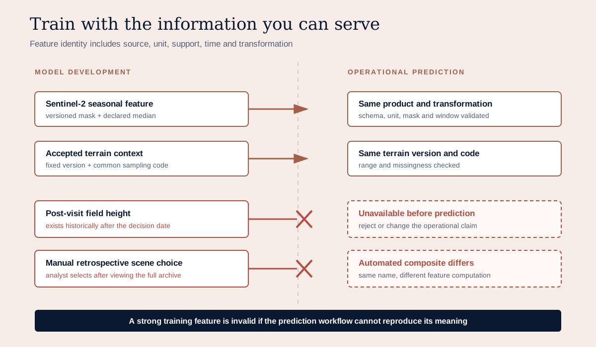
Training-serving skew occurs when the features used to develop the model differ from the features available when predictions are generated. Two forms matter here:

Schema skew

Names, types, units, categories, band order or missing-value representations differ. The model expects uav_height_p95_m but receives centimetres, or the trained array order changes.

Feature-computation skew

The same feature name is produced differently. Training uses plot summaries from a cloud-free hand-selected image, while operation uses an automated seasonal composite. Both columns may be called ndvi_median, but they do not represent the same computation.

The prevention is conceptual before it is technical: define one feature contract and use the same transformation logic for development and prediction.

Check your understandingA field height measured after the monitoring date strongly predicts the target in training. Is it eligible for an operational prediction made before field visits?

Choose one answer

No; it is unavailable at prediction time and creates training-serving skewYes; strong correlation makes every predictor validYes; field variables are always preferable to EO variables

Check answer

5. Scientific rationale does not mean causal proof

A predictor hypothesis should explain why information could be present. It should not promise a mechanism the model cannot test.

Compare:

Overclaim: “NDVI controls vegetation height, so it is included.”

Predictive rationale: “Within the declared optical product and seasonal window, NDVI may act as a proxy for green canopy cover and vigour associated with vegetation height. Saturation, soil background, water and phenology may weaken or reverse this relationship.”

The second statement is more useful for later diagnostics. It predicts where the relationship may fail and what subgroup evidence to inspect.

Check your understandingA texture metric predicts habitat condition. What is the cautious interpretation?

Choose one answer

Texture may act as a proxy carrying useful predictive informationTexture is proven to cause habitat conditionTexture has no scientific limitations because it is numeric

Check answer

6. Predictor eligibility gate

Before model fitting, each candidate must pass these questions:

Gate	Question	Blocker example
identity	is the feature name and version stable?	index1 with no formula
meaning	what measurement or transformation does it represent?	band values with unknown scaling
support	does its ground and time support match the target contract?	annual composite for a short-lived target without justification
provenance	can the source and derivation be reproduced?	manually copied values
availability	will it exist when predictions are needed?	field measurement collected afterward
consistency	will training and prediction use the same computation?	manual versus automated mask
leakage	does it directly or indirectly contain target information?	target-derived condition score
quality	how are missing, invalid and low-quality values handled?	clouds encoded as reflectance zero
domain	where could the relationship change?	sensor- or site-specific proxy

A predictor can be marked:

• eligible;
• eligible with conditions;
• diagnostic only;
• blocked;
• rejected.

Preserve rejected candidates and reasons. A transparent exclusion is part of the scientific method.

7. Worked example — enforce operational availability

Predict before running

Predict which candidate will be rejected. Would removing it prove the remaining predictors are valid?

candidates = [
    {"name": "sentinel2_ndvi", "available": True},
    {"name": "uav_height_p95", "available": True},
    {"name": "post_visit_field_height", "available": False},
]

eligible = []
for predictor in candidates:
    if not predictor["available"]:
        print("REJECT", predictor["name"], "not available at prediction time")
        continue
    eligible.append(predictor["name"])

print("eligible:", eligible)

Code walkthrough

1. candidates is a list because each predictor has the same review fields and order is useful for inspection.
2. Each dictionary has a stable name and an availability decision.
3. The two EO candidates are available under the synthetic workflow assumptions.
4. The post-visit field measurement is unavailable for a prediction made before the visit.
5. eligible begins empty and will contain names that pass this one gate.
6. The loop inspects each candidate.
7. not detects a false availability value.
8. The rejection message states the name and reason.
9. continue moves to the next candidate without adding the rejected feature.
10. Accepted names are appended.
11. The final output provides the candidate feature list for review.

This code checks only availability. It does not check source identity, support, leakage, quality or scientific rationale. A complete feature gate cannot be reduced to one Boolean.

Diagnostic check

Change the unavailable feature’s Boolean to True. The code accepts it, but reality has not changed. This shows why a machine-readable contract needs human-reviewed evidence. A validator can enforce a declared rule; it cannot prove the declaration is honest.

8. Training-serving skew beyond missing predictors

Operational availability includes more than the existence of a column.

Time

Will the correct observation be available by the decision deadline? A cloud-free annual composite completed in December cannot support an alert required in June.

Coverage

Will the predictor cover every intended cell? UAV structure may exist only for a few surveyed sites, while Sentinel imagery covers the whole domain.

Product version

Will the same collection, processing level, scaling and mask logic remain available? Record product identity and update policy.

Transformation

Will the same aggregation, resampling and missing-value logic run? Reusing a feature name does not guarantee equivalence.

Governance

Can the operational organisation legally and technically access the data? A private research layer may be unsuitable for a public annual workflow.

9. Model clinic — the strongest predictor arrives after the decision

Situation: a field-derived moisture score yields the largest performance improvement. The monitoring map must be produced one week before field visits, and the score is collected during those visits.

Question	Diagnosis
problem	the feature exists in historical training data but not at the required prediction time
evidence	workflow timeline, acquisition protocol, feature timestamp and decision deadline
consequence	the developed model cannot produce the advertised operational result
fix	reject the feature, change the decision timing, or define a separate post-field model

Do not label the field score “optional” and allow it to disappear silently. Models trained with and without it are different artefacts and need separate evaluation.

10. Common mistakes and recovery

More predictors must be better

• Why it happens: extra columns appear to provide extra information.
• How to detect it: candidates have no hypotheses or operational role.
• How to prevent it: require a rationale and limitation for every feature.
• Consequence: noise, instability and leakage become harder to diagnose.

Selecting from the final test set

• Why it happens: the team removes features that lower final-test performance.
• How to detect it: feature decisions cite final-test scores.
• How to prevent it: freeze the final test set and select only inside development folds.
• Consequence: test performance is optimistically biased.

Assuming EO predictors are direct ecological measurements

• Why it happens: variable names such as “vegetation index” sound biological.
• How to detect it: rationale omits sensor, atmosphere, support and proxy limitations.
• How to prevent it: trace measurement formation and name the hypothesised link.
• Consequence: transfer failure is misread as ecological change.

Using site ID as an innocent feature

• Why it happens: categorical site labels improve within-site predictions.
• How to detect it: performance collapses for a completely new site.
• How to prevent it: decide whether the claim is conditional on known sites and validate accordingly.
• Consequence: the model memorises location structure instead of transferable evidence.

Automatically deleting correlated variables

• Why it happens: one threshold is easy to automate.
• How to detect it: deletion ignores scientific role, stability and operational cost.
• How to prevent it: compare documented feature sets inside the same validation design.
• Consequence: useful information may be lost, while the remaining proxy is treated as uniquely important.

Allowing inconsistent feature computation

• Why it happens: training is exploratory and operation is automated later.
• How to detect it: the two pipelines cannot reproduce the same features for the same observations.
• How to prevent it: share transformation code and validate schema, units and distributions.
• Consequence: performance fails even when the fitted model file is unchanged.

11. Guided practice — audit the candidate register

Download predictor_candidate_register.csv and predictor_hypotheses_template.csv.

1. Link every candidate to the Lesson 3.2 target contract.
2. State its source, unit, spatial support and temporal support.
3. Write the expected predictive relationship without causal language.
4. Classify its role: direct measurement, proxy, nuisance, identifier, diagnostic or suspected leakage.
5. Record whether it exists at prediction time and how it will be computed.
6. Identify correlated or overlapping feature families.
7. State one known limitation and one condition likely to change the relationship.
8. Assign an eligibility status and evidence-based reason.

Include at least one rejected predictor. A register containing only accepted features has probably hidden part of the decision process.

Check your understandingTwo indices are strongly correlated. What should happen immediately?

Choose one answer

Document their roles and evaluate redundancy and stability within validationDelete one using an automatic universal thresholdKeep both and claim they are independent mechanisms

Check answer

12. Independent challenge — create predictor_hypotheses.csv

Use these exact fields:

predictor
source
unit
spatial_support
temporal_support
scientific_rationale
expected_relationship
known_limitation
available_at_prediction_time
operational_derivation
role
eligibility_status
decision_reason

Requirements:

• 8–14 candidate predictors;
• at least three EO measurement families;
• one nuisance or acquisition variable;
• one diagnostic-only field;
• one deliberate rejection for leakage or operational unavailability;
• no undocumented transformation names;
• no feature selected solely because it “should improve accuracy.”

Add a short FEATURE_SET_DECISION.md that names the primary feature set and two alternatives to compare later: a simpler operational set and a fuller research set. Do not compare their performance yet.

13. Scientific interpretation

The predictor register is not a list of proven ecological drivers. It is a set of testable predictive hypotheses and operating constraints. Later validation will determine whether the relationships persist for relevant new cases. Later interpretation will examine which conclusions are stable. Neither step converts importance into causality.

The best predictor set may be smaller than the available dataset. It may favour features that are reproducible across years and organisations over features that yield a marginal development-score increase.

14. Reflection, submission and portfolio artifact

Reflection

1. Which predictor in your register is the most indirect proxy?
2. Which feature is most vulnerable to time mismatch?
3. Could a site or campaign identifier create memorisation?
4. Which pair is most redundant, and what evidence will you examine later?
5. Can the complete primary feature set be generated before the decision deadline?

Submission

Submit:

• predictor_hypotheses.csv;
• FEATURE_SET_DECISION.md;
• one annotated training-serving-skew diagram;
• a 250–350 word explanation of one accepted proxy and one rejected feature.

Portfolio artifact

Artifact 3.3 — Operational Predictor Hypothesis Register

This register becomes the feature contract for later baseline, XGBoost, interpretation and raster-inference work. Changes must be versioned and justified within development evidence, never based on repeated viewing of final-test results.

15. Core references and advanced reading

• scikit-learn common pitfalls: preprocessing and leakage
• Google Rules of ML: training-serving skew
• Google production ML monitoring
• Shmueli (2010), To Explain or to Predict?

Tested software versions

Python 3.12.13, NumPy 2.4.2, pandas 2.2.3, scikit-learn 1.9.0 and XGBoost 3.3.0. The worked example uses core Python so that the predictor decision remains independent of a model API.