Terrain Analysis with DEM and DSM

1. Name the surface before calculating its slope

Learning outcome

By the end of this lesson, you will be able to distinguish DEM, DSM and DTM terminology; audit horizontal and vertical reference information; derive slope, aspect and hillshade from a gridded elevation surface; explain resolution and edge effects; and evaluate whether a DSM–DTM difference is interpretable without calling it vegetation height automatically.

Prerequisites: Complete Lessons 2.2, 2.11–2.14 and 2.16. You should understand horizontal CRS, raster alignment, continuous resampling, NoData and neighbourhood processing. Allow 110–140 minutes. This is a scientific application lab.

Why this matters

Terrain variables shape water movement, inundation, solar exposure and vegetation patterns. They are widely used as predictors in ecological and Earth Observation models. They are also easy to misinterpret.

A slope calculated from a canopy-following surface is not necessarily terrain slope. A height difference between two unaligned products can show grid shift rather than vegetation structure. An elevation value in metres is incomplete without a vertical reference. A beautiful hillshade is illumination modelling, not an independent measurement.

Terrain principle: Derivatives inherit the surface meaning, units, reference, resolution, uncertainty and artefacts of their elevation input.

Scientific context

The synthetic training pack includes training_dem.tif and training_dsm.tif. They share the same EPSG:3301 horizontal grid and both store synthetic values labelled in metres. Their vertical datum is deliberately undocumented, so they cannot be described as metres above sea level.

The DSM includes a small constructed upper-surface feature. This allows alignment and differencing exercises. It is not a measured canopy and must not be presented as published Baltic meadow vegetation height.

Learner action

Create 07_terrain_analysis.ipynb. Before opening the files, make a surface-register table with columns file, surface intended, horizontal CRS, vertical reference, units, date, resolution, NoData, source method and permitted interpretation. Mark unknowns as unknown.

2. DEM is a broad term

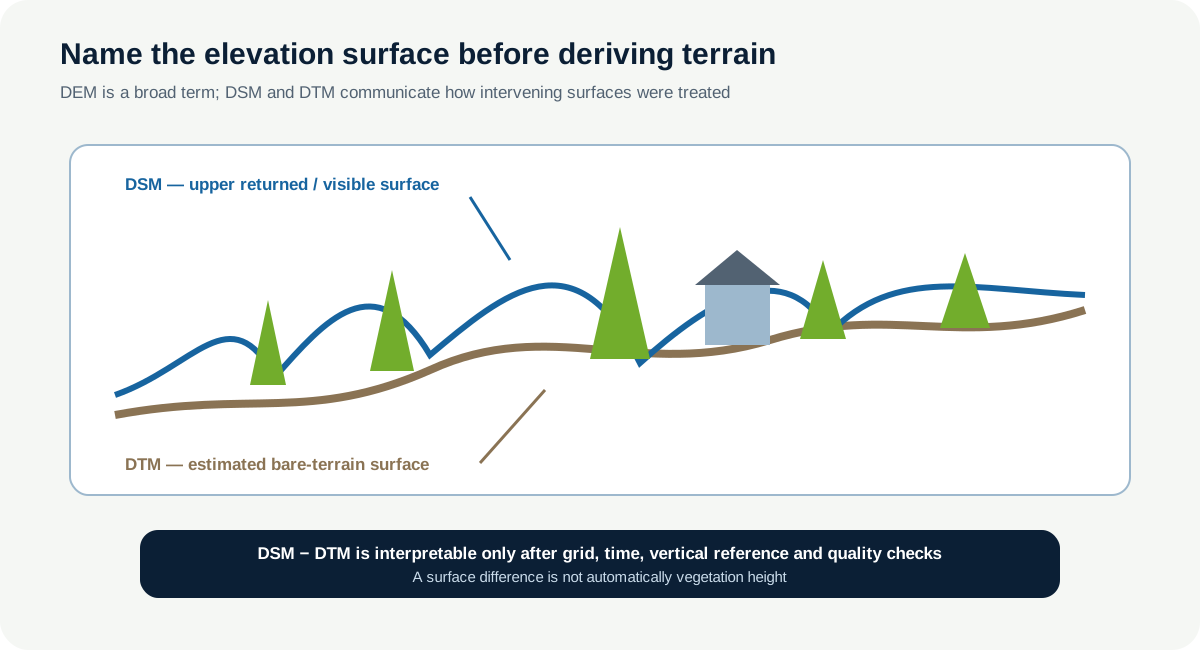
Digital elevation model (DEM) is often used as a general term for gridded elevation surfaces. Product communities also use more specific terms:

• Digital surface model (DSM): represents an upper visible or returned surface influenced by terrain, vegetation, buildings and the sensing/processing method.
• Digital terrain model (DTM): attempts to represent bare terrain after ground classification, interpolation or another explicit surface-generation process.

Usage can vary across organisations. Do not infer the surface from the acronym alone. Read the product definition and processing lineage.

A UAV photogrammetric DSM may follow plant canopy, bare patches, infrastructure, water artefacts and reconstruction noise. A LiDAR-derived DTM depends on ground-point classification and interpolation. Neither is the physical surface itself; both are modelled observations with scale and uncertainty.

Check your understandingWhat does a DSM usually attempt to represent?

Choose one answer

An upper visible or returned surface influenced by terrain, vegetation, structures and processingGuaranteed bare terrainVegetation height independent of a terrain reference

Check answer

3. Horizontal and vertical reference answer different questions

The horizontal CRS locates cells across Earth. The vertical reference explains what an elevation is measured relative to.

Record:

• horizontal CRS and axis units;
• vertical units;
• vertical datum or reference surface;
• ellipsoidal or orthometric height convention where known;
• geoid model or transformation applied;
• acquisition and processing date;
• sensor and surface-generation method.

Ellipsoidal heights from GNSS and orthometric heights related to a gravity-based surface are not interchangeable. Two rasters can share EPSG:3301 horizontally while using different or unknown vertical references.

Do not write “metres above sea level” from a UNITS=metres tag. Units provide a scale; the datum provides the reference. If the reference is absent, report “stored in metres; vertical reference undocumented” and restrict interpretation.

Check your understandingA raster tag says elevation units are metres, but no vertical datum is documented. What can be claimed?

Choose one answer

Stored vertical values use a metre scale, but their reference surface remains undocumentedEvery value is metres above sea levelThe raster can be subtracted from any other metre-valued elevation product

Check answer

4. Slope is rate of elevation change

Slope describes the magnitude of the local elevation gradient. If dz/dx and dz/dy are elevation change per horizontal distance, gradient magnitude is:

sqrt((dz/dx)² + (dz/dy)²)

Slope can be reported as:

• degrees: angle from horizontal, atan(gradient) converted to degrees;
• percent: gradient × 100.

Label the unit. A 45-degree slope equals a 100 percent grade; the numbers are not interchangeable.

Horizontal and vertical units must be compatible. If elevation is centimetres and grid spacing is metres, convert one before calculating. Otherwise the gradient is scaled by 100. Geographic degrees are not metre distances; use a suitable projected grid or a method that handles geodesic spacing.

Slope is a neighbourhood derivative. Cells beside NoData and dataset edges lack a complete neighbourhood under common finite-difference methods. Record edge treatment and mask affected outputs.

5. Aspect is circular direction

Aspect describes the direction of steepest descent, commonly expressed as a compass bearing clockwise from north:

• 0° or 360°: north;
• 90°: east;
• 180°: south;
• 270°: west.

Conventions vary, so store the definition. Flat cells have undefined aspect; assigning them zero falsely labels them north-facing.

Aspect is circular. One degree and 359 degrees differ by two degrees, not 358. An ordinary arithmetic mean can be misleading. Circular summaries or transformed components such as sine and cosine may be needed in later modelling.

Aspect interpretation also depends on hemisphere, season, topographic shading and ecological mechanism. A direction is not itself solar exposure.

Check your understandingWhy should ordinary arithmetic not average aspects 1° and 359°?

Choose one answer

Aspect is circular, so the two directions are only two degrees apartAspect has no unitsOne of the two values must be NoData

Check answer

6. Worked example — derive slope and aspect explicitly

Predict before running

The synthetic DEM rises mainly as row number increases and slightly as column increases. Which compass direction should the steepest downhill direction favour? Predict the approximate slope range before running.

import numpy as np
import rasterio

with rasterio.open("data/raw/training_dem.tif") as src:
    dem = src.read(1, masked=True).filled(np.nan)
    xres, yres = abs(src.res[0]), abs(src.res[1])

dz_drow, dz_dx = np.gradient(dem, yres, xres)
slope = np.degrees(np.arctan(np.hypot(dz_dx, dz_drow)))
aspect = (np.degrees(np.arctan2(-dz_dx, dz_drow)) + 360) % 360
aspect[np.isclose(slope, 0) | ~np.isfinite(slope)] = np.nan

print(np.nanmin(slope), np.nanmax(slope))
print(np.nanmin(aspect), np.nanmax(aspect))

Code walkthrough

1. Rasterio supplies the gridded elevation values and pixel dimensions.
2. The masked array is filled with NaN for floating calculations; it is not filled with zero elevation.
3. Absolute resolution values provide positive horizontal distances.
4. np.gradient estimates change along increasing row and column directions.
5. Gradient magnitude combines the two components.
6. arctan converts rise/run to slope angle.
7. The aspect formula converts the downhill vector to a clockwise-from-north bearing for this north-up row convention.
8. Aspect becomes NaN for flat or invalid cells.
9. Minimum and maximum exclude invalid values.

This compact example is educational. A production terrain algorithm must document finite-difference method, neighbourhood, edge behaviour, rotated grids and z-factor. Compare with a trusted GIS implementation on a known fixture.

7. Hillshade is a visual model

Hillshade simulates illumination from a chosen azimuth and altitude using slope and aspect. It is excellent for revealing terrain artefacts, pits, stripes and edge seams. It is not a measured terrain variable and should not be used as an ecological predictor without a separate physical rationale.

azimuth = np.radians(315)
altitude = np.radians(45)
slope_rad = np.radians(slope)
aspect_rad = np.radians(aspect)

illumination = (np.sin(altitude) * np.cos(slope_rad) +
                np.cos(altitude) * np.sin(slope_rad) *
                np.cos(azimuth - aspect_rad))
hillshade = np.clip(255 * illumination, 0, 255)
hillshade[~np.isfinite(slope)] = np.nan

Changing azimuth or altitude changes the image without changing the surface. Store illumination parameters in the figure caption. Do not interpret dark cells as low elevation; they are cells facing away from the modelled light or affected by the renderer and mask.

8. Resolution changes the derivative

Terrain derivatives depend on grid spacing and preprocessing. A fine DSM can contain canopy texture and reconstruction noise, producing steep local gradients. A coarser grid smooths that variation. Resampling before slope changes the surface and therefore the derivative.

Record:

• native surface resolution;
• any resampling method;
• target derivative resolution;
• smoothing or filtering;
• neighbourhood method;
• NoData and edge treatment;
• whether the result describes terrain, upper surface or another model.

Finer pixel size does not prove more accurate slope. A high-resolution noisy surface can produce less reliable local gradients than a validated coarser DTM for a terrain question.

Check your understandingWhat can happen when slope is derived from a finer but noisy DSM?

Choose one answer

Canopy texture and reconstruction noise can create steep local gradientsFiner cells guarantee more accurate terrain slopeResolution removes the need for vertical-reference metadata

Check answer

9. DSM–DTM differencing has strict prerequisites

A surface-height approximation is sometimes calculated as:

surface difference = DSM − DTM

Interpretation requires:

• identical or explicitly harmonised horizontal grid;
• compatible vertical units and reference;
• compatible acquisition time;
• DSM that represents the relevant upper surface;
• DTM that reasonably represents underlying terrain;
• independent validation of both surfaces and the difference;
• treatment of buildings, water, gaps and reconstruction artefacts.

Only under appropriate conditions might the difference be called a canopy-height model. Even then, it may not equal field vegetation height. In coastal meadows, low vegetation, microtopography and photogrammetric noise can have similar magnitude.

Use the Lesson 2.14 alignment validator before subtraction. Report negative differences and unexpected spikes instead of clipping them silently. They can reveal reference, alignment or modelling problems.

10. Terrain QA combines numerical and visual evidence

Before accepting derivatives, report:

• source checksum and surface type;
• horizontal and vertical reference status;
• units and resolution;
• CRS, transform, shape, bounds and NoData;
• slope unit and plausible range;
• undefined aspect count;
• hillshade illumination settings;
• derivative edge mask;
• alignment evidence for any differencing;
• representative profiles or transects;
• comparison with independent control or authoritative terrain evidence where available.

QGIS hillshade and profile views can reveal stripes, pits, steps and tile seams. Use them for diagnosis. A visually smooth surface can still have a vertical bias, so visual QA cannot replace checkpoints or reference validation.

11. Common mistakes and recovery

Treating DSM as bare terrain

Why it happens: both store elevation-like values. Recognition: vegetation and structures are ignored in interpretation. Fix: inspect the product definition and call the surface what the evidence supports.

Calling stored metres “above sea level”

Why it happens: units are confused with reference. Recognition: no vertical datum or geoid information is recorded. Fix: report units and vertical-reference status separately.

Mixing horizontal and vertical units

Why it happens: slope code accepts any numbers. Recognition: implausible near-vertical slopes appear on gentle ground. Fix: convert units explicitly and record the z-factor.

Averaging aspect linearly

Why it happens: bearings are stored as ordinary numbers. Recognition: 1° and 359° average to 180°. Fix: use circular statistics or sine/cosine components.

Interpreting hillshade as measurement

Why it happens: shaded relief resembles topography. Recognition: hillshade values enter a model as elevation evidence. Fix: label it as illumination-based visual QA and retain source derivatives separately.

Subtracting unaligned surfaces

Why it happens: arrays have the same shape. Recognition: transform, vertical reference or dates were not compared. Fix: run complete alignment and compatibility checks before differencing.

Equating DSM–DTM with vegetation height

Why it happens: a positive surface difference appears canopy-like. Recognition: no surface-generation or field validation evidence exists. Fix: call it a surface difference until conditions and validation support a stronger interpretation.

12. Guided practice — derive and review terrain products

Use training_dem.tif and training_dsm.tif.

1. verify checksums and complete surface metadata records;
2. state that the horizontal CRS is known and vertical datum is undocumented;
3. confirm exact grid alignment before any subtraction;
4. read the DEM as a masked array;
5. calculate slope in degrees and label the unit;
6. calculate aspect with undefined flat and invalid cells masked;
7. calculate one hillshade with recorded azimuth and altitude;
8. mask derivative cells whose neighbourhood touches NoData where required;
9. write each derivative with source, method and unit tags;
10. reopen and verify grid, NoData, valid counts and plausible ranges;
11. calculate training_dsm - training_dem only as a synthetic surface difference;
12. report negative values, maximum difference and limitations;
13. create a QA map and one elevation profile;
14. export terrain_derivative_report.csv.

Raster QA check

Load the two surfaces, slope, aspect and hillshade in QGIS. Confirm raster properties and use nearest-neighbour display while inspecting raw cells. Change hillshade illumination to prove that display changes without a new elevation observation. Inspect derivative edges and the constructed DSM feature. Record every renderer parameter used in the QA figure.

13. Independent challenge — assess a proposed vegetation-height product

A collaborator proposes subtracting a 2024 UAV DSM from a 2018 regional terrain model and labelling the result “vegetation height.” Write a professional review:

• compare horizontal and vertical references;
• compare grid, resolution, extent and alignment;
• compare acquisition times and surface-generation methods;
• identify land-cover and building effects;
• specify independent field validation;
• propose sensitivity checks for co-registration and terrain error;
• define an acceptable output name before validation;
• state conditions under which the product must be rejected.

Do not solve the problem by resampling alone. Resampling can align representation while preserving source uncertainty and temporal mismatch.

Scientific interpretation

Terrain derivatives describe the local geometry of a declared elevation surface under a declared method. They do not independently verify that surface, identify ecological causation or remove vertical uncertainty. A DSM slope can be useful, but it may describe canopy and reconstruction texture rather than ground terrain.

14. Reflection, submission and portfolio artifact

Answer in your private notes:

1. Why is DEM a broad term?
2. What is missing when only “metres” is documented?
3. Why is aspect circular and undefined on flat cells?
4. How does raster resolution affect slope?
5. Which evidence is required before DSM–DTM can be called vegetation height?

Submission

• Notebook: 07_terrain_analysis.ipynb with surface audit, slope, aspect, hillshade, surface-difference review and independent challenge.
• Table: terrain_derivative_report.csv containing source, method, unit, range, mask and reference fields.
• Screenshot: QGIS terrain QA layout with surface type, illumination parameters and vertical-reference limitation visible.
• Written answer: 260–340 words interpreting one derivative and explaining what the available metadata cannot support.

Portfolio artifact

Artifact 2.17 — Terrain derivative and interpretation report

Add the verified derivatives, method record and limitation statement to the Raster QA and Harmonisation Pipeline. The artifact demonstrates that terrain computation and terrain interpretation remain linked but distinct professional tasks.