Raster–Vector Integration

1. Begin with the field measurement, not the extraction API

Learning outcome

By the end of this lesson, you will be able to choose among point sampling, plot-footprint extraction, a justified buffer and zonal statistics; compare their spatial support; report valid-cell count and coverage fraction; handle NoData without substituting zero; and produce a traceable raster-extraction table for synthetic plot polygons.

Prerequisites: Complete Lesson 2.3 on spatial support, Chapter 2 vector geometry and Lessons 2.11–2.14 on raster grids and alignment. Allow 120–150 minutes. This is a scientific practicum.

Why this matters

Raster–vector extraction converts a spatial field into rows that look ready for statistics. A plot receives one reflectance value, a polygon receives a mean, and the table joins to ecological measurements. The ease of producing the table can hide the most important decision: what ground area contributed to each value?

A one-square-metre clipped-biomass quadrat, a GNSS point and a ten-metre raster cell do not have the same support. Extracting the nearest cell is not neutral. Averaging a large buffer is not automatically safer. The extraction method defines the quantity that enters the analysis.

Support principle: Ask what the field observation represents, then select raster support that answers a comparable scientific question.

Scientific context

The published Baltic plant-traits table does not supply public plot coordinates. This lesson therefore uses training_plot_polygons.geojson, a synthetic WGS 84 vector file, and the synthetic continuous raster. The polygons are designed to overlap known grid cells after transformation to EPSG:3301.

The exercise teaches method. It does not attach synthetic pixels to published ecological samples or claim that the training values are real reflectance.

Learner action

Create 05_raster_vector_integration.ipynb. Before opening a raster, write a support statement for four hypothetical field records: point observation, 1 m² quadrat, 30 m plot polygon and uncertain GNSS location. For each, name what is observed and what is only a coordinate representation.

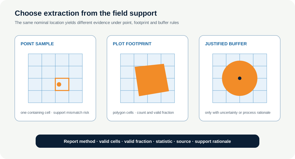
2. Point sampling selects the containing cell

Point sampling converts an x/y coordinate to a raster row and column and returns that cell's value. It is simple and reproducible when CRS and transform are correct.

It can be defensible when:

• the target itself is effectively point-like at the analysis scale;
• the cell value is intended to represent the point location;
• geolocation uncertainty is small relative to homogeneous surroundings;
• the scientific question asks for the containing-cell value.

Risks include:

• the point represents the centre of a larger field footprint;
• a small positional error selects another cell;
• the point lies near a class or NoData boundary;
• the raster cell is much larger or smaller than the observation support;
• one cell contains mixed land cover.

“Nearest pixel” can also mean nearest centre rather than containing cell. State the rule. A coordinate exactly on a cell edge requires a consistent convention.

Check your understandingWhen is a containing-cell point sample most defensible?

Choose one answer

When the observation and question are point-like at the analysis scale and positional uncertainty is acceptableWhenever it gives the strongest relationshipWhenever the raster has smaller pixels than the field plot

Check answer

3. Plot-footprint extraction respects known area

When a field plot polygon is known, select cells contributing to that footprint. This creates several design choices:

• include cells whose centres fall inside;
• include all touched cells;
• weight cells by overlap area;
• rasterise the polygon onto a finer support grid;
• require complete or minimum valid coverage.

A centre-in-polygon rule is reproducible and efficient, but it can exclude narrow edge contributions. all_touched=True can over-represent boundary cells, especially when cells are large relative to the polygon. Exact area weighting more closely represents geometric overlap but still assumes the raster value is uniform within each cell and the polygon geometry is accurate.

Report the rule with the statistic. “Plot mean” is incomplete without explaining which cells and weights created it.

4. A buffer needs scientific or uncertainty justification

A buffer creates a neighbourhood around a point or footprint. It may be useful when:

• positional uncertainty is quantified and the buffer supports a sensitivity analysis;
• the measured ecological process genuinely represents a neighbourhood;
• sensor point-spread or georegistration evidence motivates an extraction support;
• a published protocol defines the radius.

It is not justified merely because a larger sample has lower variance or a stronger correlation. A 2 m buffer around a point is not the same as a 2 m uncertainty distribution. All locations inside the buffer are usually weighted equally unless another rule is implemented.

Use projected metre units, preserve the unbuffered geometry and test plausible radii chosen before reviewing the ecological result.

5. Zonal statistics summarise selected cells

Common zonal statistics include:

• count of valid cells;
• mean or area-weighted mean;
• median;
• minimum and maximum;
• standard deviation;
• class counts or proportions;
• valid fraction.

Do not calculate all statistics by default. Each answers a different question. Mean estimates the arithmetic average of selected values and is sensitive to extremes. Median estimates the middle selected value and changes the estimand. Standard deviation describes within-zone variation only under the selected support and does not equal measurement uncertainty.

For categorical rasters, a numeric mean of class codes is usually meaningless. Report class counts, area proportions, mode or diversity only with a clear legend and tie rule.

Check your understandingWhich summary is appropriate for categorical habitat codes?

Choose one answer

Class counts or proportions with a documented legend and tie ruleThe arithmetic mean of class identifiersA bilinear value at the polygon centroid

Check answer

6. CRS and grid alignment come before extraction

Transform vector geometry to the raster CRS; do not relabel it. Check raster transform, valid-data mask and bounds. Then confirm that the geometry overlaps the declared extent.

Use the raster grid as the extraction reference. A vector polygon has effectively continuous coordinates; rasterisation assigns that geometry to discrete cells. The rasterisation rule is part of the method.

If several raster predictors will be extracted together, align them first. Otherwise, the same polygon can select different ground cells across layers, and a row of extracted values will not necessarily describe one support.

7. Positional uncertainty and edge effects can dominate

Fine-resolution rasters are especially sensitive to position. A 0.5 m GNSS error crosses ten 5 cm UAV cells. A plot near water, bare soil or a habitat boundary can receive very different values under small shifts.

Create diagnostics for:

• distance from plot centre or boundary to raster discontinuities;
• extraction under plausible x/y shifts;
• alternative footprint and buffer rules;
• proportion of cells from each class;
• valid coverage at edges;
• temporal mismatch between field and image.

Do not hide edge cases by dropping them. Flag them and decide whether they require exclusion, a robust summary, uncertainty propagation or a separate analysis stratum.

Check your understandingWhy must valid fraction accompany a plot mean?

Choose one answer

The statistic may describe only a small valid part of the intended footprintIt proves the raster is positionally accurateIt converts missing cells to zero

Check answer

8. Valid coverage belongs in every output row

Suppose a polygon intersects nine raster cells, but only five are valid. A mean calculated from those five may represent the remaining visible area, not the complete plot.

Report:

• total candidate or intersected cells under the rule;
• valid cell count;
• valid fraction;
• reason for invalidity when known;
• threshold used for acceptance;
• statistic only when the threshold passes, or an explicit review status.

A rule such as minimum_valid_fraction = 0.8 must be justified from product quality and analysis purpose. Do not choose it to maximise sample size. Run a sensitivity analysis if several thresholds are defensible.

Never replace a missing extraction with zero. Zero can be a valid value and would falsely imply measurement evidence where none exists.

9. Worked example — select valid cells inside a polygon

Predict before running

Will the output mean include NoData? Which object determines the selected footprint: the polygon, its bounding box or its centre?

import numpy as np
import rasterio
from rasterio.features import geometry_mask

with rasterio.open("data/raw/aligned_continuous.tif") as src:
    band = src.read(1, masked=True)
    inside = geometry_mask([plot_geometry], out_shape=src.shape,
                           transform=src.transform, invert=True)
    candidate_count = int(inside.sum())
    valid_inside = inside & ~np.ma.getmaskarray(band)
    values = band.data[valid_inside]

print("valid cells:", values.size)
print("valid fraction:", values.size / candidate_count)
print("mean:", values.mean() if values.size else None)

plot_geometry must already be a valid GeoJSON-like geometry in the raster CRS. This example uses the default centre-based rasterisation behaviour. It does not calculate area weights.

Code walkthrough

1. NumPy supports explicit mask combination.
2. Rasterio reads the grid and rasterises vector geometry.
3. masked=True preserves source validity.
4. geometry_mask() creates a Boolean grid under the declared geometry rule.
5. invert=True makes cells inside the polygon True.
6. Candidate count records geometrically selected cells before source validity.
7. The source mask is inverted so only valid cells remain.
8. Values are selected from the data only where both conditions are true.
9. Valid count and fraction accompany the statistic.
10. Empty support returns None rather than a false zero.

10. Compare methods before selecting one

For each synthetic plot, calculate:

1. containing-cell point sample at the centroid;
2. polygon centre-based mean;
3. polygon centre-based median;
4. 2 m buffered-polygon mean;
5. valid count and valid fraction for every polygon rule.

Expect different answers. The question is not which number looks most ecological. Explain why the support changed and which method matches the hypothetical field protocol.

Centroid point sampling can be especially misleading for concave or multipart plots. A centroid can lie outside the polygon. Use a verified field location when the protocol defines one; do not manufacture an observation point from geometry and call it measured.

11. Design the extraction table as an evidence product

plot_raster_extraction.csv must include at least:

• plot_id;
• source geometry file and checksum;
• raster source and checksum;
• raster band, variable and units;
• extraction method;
• geometry support and buffer radius if used;
• rasterisation or weighting rule;
• valid cell count;
• candidate cell count;
• valid fraction;
• statistic name and value;
• image and field dates or temporal support;
• CRS and grid identifier;
• positional-uncertainty note;
• acceptance or review status.

Rows should remain traceable to immutable inputs. The table is not merely model input; it is the record of how spatial evidence became tabular evidence.

12. Common mistakes and recovery

Taking the nearest pixel by default

Why it happens: point sampling is easy. Recognition: no field footprint or uncertainty rationale exists. Fix: describe the observation support first and compare defensible alternatives.

Averaging class codes

Why it happens: zonal statistics expose a mean option for any numeric raster. Recognition: habitat classes produce values such as 1.8. Fix: use class counts or proportions with the documented legend.

Ignoring valid coverage

Why it happens: the mean function returns a number. Recognition: cell count and fraction are absent. Fix: report coverage and apply a predeclared acceptance rule.

Treating a buffer as uncertainty

Why it happens: a radius looks like a positional interval. Recognition: all buffered cells receive equal weight without an uncertainty model. Fix: state whether the buffer represents support, sensitivity or an approximation and avoid overstating it.

Extracting from unaligned predictors

Why it happens: every raster overlaps the plot visually. Recognition: transforms differ across extracted bands. Fix: prove grid alignment or document a support-specific extraction strategy before combining rows.

Replacing missing output with zero

Why it happens: models reject nulls. Recognition: zero appears where valid count is zero. Fix: retain missingness, explain why it occurred and handle it transparently downstream.

13. Guided practice — compare four extraction supports

Use the synthetic plot polygons and continuous raster.

1. record checksums, CRS and support semantics;
2. transform polygons from WGS 84 to EPSG:3301;
3. validate geometry and overlap with raster bounds;
4. compute centroid-containing-cell samples, clearly labelled as derived centroids;
5. compute polygon mean and median using one declared rasterisation rule;
6. compute a 2 m buffer mean only as a sensitivity scenario;
7. report candidate and valid cells for every polygon-based method;
8. set and justify a minimum-valid-fraction rule before reviewing values;
9. compare outputs and explain each difference through support and edge behaviour;
10. write plot_raster_extraction.csv and reopen it;
11. create one map showing polygons, selected cells and NoData;
12. identify at least one limitation that no extraction method removes.

Raster QA check

In QGIS, overlay the transformed plot polygons on the raster with pixel boundaries visible. Inspect which cells each support includes. Compare QGIS zonal output with the Python table for one plot, matching rasterisation settings as closely as possible. If values differ, investigate CRS, all-touched behaviour, NoData, selected band and geometry version rather than choosing the preferred result.

14. Independent challenge — design extraction for a 1 m² quadrat

A 1 m² biomass quadrat has a verified centre with 0.7 m horizontal uncertainty. Available imagery includes a 5 cm UAV raster and a 10 m satellite band.

Write a method design that:

• distinguishes the quadrat footprint from coordinate uncertainty;
• proposes one main UAV extraction and a sensitivity analysis;
• explains why one UAV pixel is insufficient;
• explains why one satellite cell is a support mismatch;
• proposes how multiple quadrats or homogeneous areas could support satellite validation;
• specifies valid-coverage and temporal rules;
• states how registration uncertainty will be reported;
• refuses any claim unsupported by the available geometry.

Do not calculate a correlation. The deliverable is the design that must precede it.

Scientific interpretation

Extraction establishes a reproducible mapping from declared vector support to valid raster cells. It does not prove the raster variable is a valid ecological proxy, eliminate geolocation uncertainty, align observation times or make supports identical. Those limitations must accompany the extracted values into later modelling.

15. Reflection, submission and portfolio artifact

Answer in your private notes:

1. When is point sampling scientifically defensible?
2. How do all-touched and centre-based rules change support?
3. Why is valid fraction part of the result rather than only QA?
4. Which zonal statistics make sense for categorical data?
5. How can positional uncertainty change a fine-resolution extraction?

Submission

• Notebook: 05_raster_vector_integration.ipynb with four methods, coverage evidence and the independent design.
• Table: plot_raster_extraction.csv containing support, validity, source and statistic fields.
• Screenshot: raster cells and vector supports shown together with selected cells visible.
• Written answer: 260–340 words defending the selected method and explaining why the alternatives differ.

Portfolio artifact

Artifact 2.15 — Spatially justified raster extraction table

Add the method record, extraction table and QA map to the Raster QA and Harmonisation Pipeline. The table becomes the controlled bridge between spatial observations and later ecological modelling.

From the Field — extraction creates a model row

Use plot geometry and a documented support rule to extract UAV values for each SampleID. Do not turn many pixels inside one plot into independent field observations: the quadrat remains the observational unit. See how plot responses meet UAV predictors.