Raster Alignment and Grid Integrity

1. Prove that corresponding indices describe the same ground

Learning outcome

By the end of this lesson, you will be able to determine whether rasters are genuinely compatible for cell-by-cell analysis, diagnose CRS, transform, resolution, origin, bounds, dimensions and NoData differences, design a justified target grid, and create a reusable alignment report that fails clearly on deliberate mismatches.

Prerequisites: Complete Lessons 2.11–2.13. You should understand affine transforms, crop, mask, reprojection and variable-specific resampling. Allow 130–150 minutes. This is a professional practicum.

Why this matters

Raster arithmetic is deceptively easy. NumPy will subtract two arrays with the same shape. A machine-learning table can place two flattened bands side by side. Neither operation knows whether cell [4, 7] in both arrays describes the same square of ground.

Misalignment can create believable but false spectral indices, surface differences and predictor stacks. A half-cell shift mixes neighbouring supports everywhere. The output can remain smooth enough to escape visual review.

Alignment principle: For cell-wise analysis, every corresponding row and column must represent the same ground footprint under a compatible measurement contract.

The following statements are all false:

• same CRS means same alignment;
• same resolution means same alignment;
• same width and height mean same grid;
• visual overlap proves cell correspondence.

Scientific context

The training pack provides controlled failures:

• aligned_continuous.tif is the reference grid;
• aligned_categorical.tif shares that grid but uses different NoData semantics;
• shifted_origin.tif has the same CRS, shape and resolution but a half-cell origin shift;
• different_crs.tif declares another CRS;
• different_resolution.tif uses 20 m cells;
• cropped_extent.tif has matching cell size and CRS but a smaller extent;
• missing_crs.tif cannot enter spatial harmonisation until provenance resolves its source CRS.

Because the cases are synthetic, the expected diagnosis is known. In real work, the same report becomes evidence for acceptance, transformation or rejection.

Learner action

Create 04_alignment_validation.ipynb. Before opening the files, make an expected-results matrix with one row per case and columns CRS, resolution, origin, shape, bounds, NoData and aligned. Commit to the prediction.

2. Alignment is a complete grid contract

Compare at least:

1. CRS: equivalent horizontal reference definition, not only similar display names;
2. affine transform: origin, x/y steps, rotation and shear;
3. resolution: x and y grid spacing in CRS units;
4. origin: where the lattice begins;
5. bounds: outer grid edges;
6. dimensions: height and width;
7. pixel orientation: north-up or rotated/sheared geometry;
8. NoData and mask policy: which cells can participate;
9. band meaning and units: whether cell-wise combination is scientifically meaningful;
10. temporal support: whether the observations can answer the same temporal question.

The first seven establish geometric correspondence. NoData and semantics establish analytical compatibility. Two rasters can be geometrically aligned but inappropriate to subtract because one stores reflectance and the other habitat labels.

Check your understandingTwo rasters share EPSG:3301 and 10 m pixels. What else is required for cell-wise alignment?

Choose one answer

Matching transform/origin, dimensions, bounds and pixel orientation under a declared toleranceOnly similar colours in QGISOnly the same number of bands

Check answer

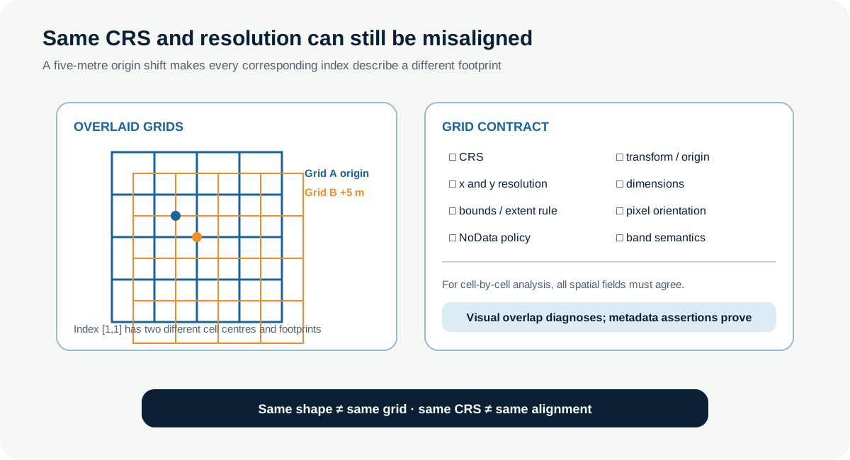
3. Grid origin controls the lattice

Consider two north-up 10 m rasters:

• Grid A origin: (500000, 6500120)
• Grid B origin: (500005, 6500125)

Both have 10 m resolution, 12 rows, 12 columns and EPSG:3301. Grid B is shifted 5 m east and 5 m north. Its cells overlap four Grid A cells rather than corresponding one-to-one.

If the arrays are combined directly, index equality becomes a false spatial assumption. No statistical technique can identify this from the values alone.

An origin difference equal to a whole number of pixels can still prevent direct stacking when bounds or dimensions differ. It may allow exact window alignment after an explicit crop. A fractional-pixel difference requires resampling to a chosen lattice.

4. Transform comparison needs an explicit tolerance

Transforms use floating-point numbers. Values derived through coordinate operations can differ by tiny numerical amounts even when they describe an intended common grid. Exact == can be too strict, while a generous tolerance can hide a meaningful shift.

Choose tolerance from:

• how the target grid was constructed;
• coordinate units;
• pixel size;
• required support correspondence;
• expected numerical precision of the software and format.

Rasterio affine transforms provide almost_equals(). Treat its precision as part of the method and supplement it with cell-centre checks. A tolerance should never be selected because it turns a failure into a pass.

For a 10 m grid, a 5 m shift is not floating-point noise. For transforms intended to be copied exactly from one reference dataset, exact coefficients or a very tight tolerance may be appropriate.

5. Worked example — return diagnostics, not one vague Boolean

Predict before running

What should the function report for the shifted-origin case? Identify the checks that pass and fail before running it.

def check_raster_alignment(reference, candidate):
    checks = {
        "same_crs": reference.crs == candidate.crs,
        "same_transform": reference.transform.almost_equals(candidate.transform),
        "same_resolution": reference.res == candidate.res,
        "same_shape": reference.shape == candidate.shape,
        "same_bounds": reference.bounds == candidate.bounds,
        "same_nodata": reference.nodata == candidate.nodata,
    }
    checks["aligned"] = all(checks[key] for key in (
        "same_crs", "same_transform", "same_resolution",
        "same_shape", "same_bounds"))
    return checks

Code walkthrough

1. The function accepts open Rasterio datasets so their metadata remain available.
2. CRS comparison checks the parsed spatial-reference objects.
3. almost_equals() compares all affine coefficients with a small numerical tolerance.
4. Resolution compares x and y steps.
5. Shape compares rows and columns.
6. Bounds compare outer grid edges.
7. NoData is reported separately because different sentinels can exist on the same geometry.
8. aligned requires the geometric fields rather than NoData equality.
9. Returning every field makes the cause actionable.

For production, add configurable tolerances, pixel orientation, masks, band units and source identity. Never reduce the result to False without explaining why.

Check your understandingWhy should an alignment function return individual checks?

Choose one answer

Property-level results expose the cause and required correctionA single False value proves the source data are scientifically invalidIt allows failed checks to be ignored silently

Check answer

6. Verify one known cell centre

Metadata assertions are the main proof. A cell-centre diagnostic makes the implication tangible:

from rasterio.transform import xy

row, col = 4, 7
reference_xy = xy(reference.transform, row, col, offset="center")
candidate_xy = xy(candidate.transform, row, col, offset="center")

print("reference:", reference_xy)
print("candidate:", candidate_xy)
print("offset:", tuple(b - a for a, b in zip(reference_xy, candidate_xy)))

For the shifted training raster, the centre offset should expose the 5 m difference in both axes. The cell-centre check does not replace full transform comparison; it illustrates one consequence for a traceable index.

7. Choose the target grid from the scientific purpose

Harmonisation requires one explicit destination contract:

• target CRS;
• resolution;
• origin;
• extent;
• dimensions;
• pixel orientation;
• NoData policy;
• resampling method per variable.

A reference raster can provide this contract. Selection still needs justification. Possible reasons include:

• it is the validated primary observation for the analysis;
• its CRS controls distortion for the study area;
• its resolution matches the intended support without pretending to add information;
• its origin follows a governed project lattice;
• its extent represents the agreed study area.

Do not choose the finest file automatically. A centimetre UAV grid may be inappropriate as the destination for a broad satellite analysis and can multiply storage without increasing the satellite evidence.

Check your understandingWhich rationale can justify a reference grid?

Choose one answer

Its CRS, support, resolution, extent and governed origin fit the stated analysisIt has the smallest cells, so it must be most accurateIt is the first file alphabetically

Check answer

8. Intersection and union answer different coverage questions

When input extents differ, define the output extent policy.

Intersection extent retains only the area covered by every required layer. It reduces missing data but can discard valid edge observations and shrink the study population.

Union extent retains the full combined coverage. Cells outside each source become NoData in that layer. It preserves spatial coverage but requires explicit missingness and may leave few complete cases at edges.

A site-boundary mask is another policy. It can be combined with intersection or union, but it does not eliminate source-specific gaps inside the site.

Report the area and valid-cell consequences before choosing. Never select intersection only because it produces a complete stack without explaining which ground was excluded.

9. Snap destination boundaries to the lattice

Grid snapping aligns output bounds to a declared origin and resolution. For a 10 m lattice, valid x edges might be 500000, 500010, 500020 and so on. A requested boundary at 500003 should not silently become the output origin if the stack must follow the project lattice.

Snapping can expand or contract the requested extent. Record the rule—floor, ceiling, nearest or intersection—and compare the snapped bounds with the site boundary. The output dimensions should be derivable from snapped bounds and resolution.

Rasterio's warp functions can write directly to the exact transform, shape and CRS taken from the reference dataset. This is stronger than reprojecting each file independently with separate defaults and hoping their outputs match.

10. NoData equality is not enough

Two datasets can both use -9999 while applying it to different cells. One can use an internal mask and no scalar NoData. A class raster can use 255 while a continuous raster uses -9999. These cases can be analytically compatible after a deliberate common-validity rule even though the stored sentinels differ.

For a stack, report:

• NoData scalar per band;
• internal and external mask presence;
• valid-cell count;
• joint valid mask across required layers;
• valid fraction by study unit;
• whether zero is valid;
• how output NoData is encoded;
• whether interpolation near invalid support was prevented.

Do not rewrite every source to a common sentinel merely to make metadata equal. Harmonise the analytical mask and document storage decisions in derivatives.

Check your understandingTwo aligned rasters use different NoData sentinels. What is the next step?

Choose one answer

Audit each mask and define a documented joint-validity policyTreat all zeros as missing in both filesDeclare the grids misaligned solely because the sentinels differ

Check answer

11. QGIS can reveal the shift, but not prove its absence

Overlay the aligned and shifted rasters with transparency and visible pixel grids. A half-cell offset should become apparent at cell edges. Toggle snapping and inspect cell centres at a declared location.

QGIS may reproject a layer on the fly for display. That can make different CRSs overlap visually while their stored grids remain incompatible. Renderer interpolation can also soften cell boundaries. Record:

• layer CRS and project CRS;
• displayed pixel size;
• renderer resampling settings;
• coordinates of the inspected cell centres;
• screenshot extent and scale.

Use the view to diagnose patterns. Use the Python alignment report as the reproducible assertion.

12. Common mistakes and recovery

Checking only CRS

Why it happens: CRS is the most familiar spatial field. Recognition: two same-CRS files are stacked without transform comparison. Fix: assert the complete geometric contract.

Checking only shape

Why it happens: NumPy arithmetic succeeds. Recognition: no Earth-coordinate evidence appears. Fix: compare transform, bounds, CRS and one cell centre before value operations.

Treating matching resolution as matching lattice

Why it happens: both files say 10 m. Recognition: origins differ by part of a cell. Fix: compare affine transforms and snap every derivative to one declared target grid.

Using an arbitrary tolerance

Why it happens: small numerical differences are inconvenient. Recognition: tolerance is chosen after a failed test. Fix: predeclare tolerance from coordinate units and grid-construction method.

Choosing the finest raster as reference

Why it happens: smaller cells appear better. Recognition: no support or accuracy rationale exists. Fix: choose from the question, observation scale, CRS and governed grid.

Trusting visual transparency

Why it happens: cell edges appear coincident. Recognition: renderer and on-the-fly transformation are not recorded. Fix: use visual QA as a companion to metadata and centre-coordinate assertions.

13. Guided practice — diagnose the training grid cases

Use aligned_continuous.tif as the proposed reference. Run a structured comparison against all seven diagnostic rasters.

1. record input paths and checksums;
2. compare CRS objects;
3. compare all affine coefficients with a predeclared tolerance;
4. compare x/y resolution, shape and bounds;
5. report origin and pixel orientation;
6. compare NoData and valid-mask counts;
7. calculate a declared cell centre and offset;
8. classify each case as aligned, geometrically incompatible, semantically incompatible or blocked by missing metadata;
9. define the transformation needed for every repairable case;
10. refuse to transform missing_crs.tif until source CRS evidence exists;
11. export raster_alignment_report.csv;
12. assert that the shifted, changed-CRS, changed-resolution and cropped cases fail for the expected reasons.

Raster QA check

Create a QGIS comparison showing the aligned and shifted rasters with nearest-neighbour display and visible cells. Add a text annotation containing the two stored origins and one cell-centre offset. Then inspect the different-CRS raster with on-the-fly transformation enabled and explain why apparent overlap is not stack compatibility.

14. Independent challenge — design a common grid

Design a target grid for Red, NIR, DSM and habitat layers whose sources differ in grid properties.

Your design must state:

• analysis question and intended spatial support;
• selected CRS and area of use;
• resolution with a non-accuracy rationale;
• origin and snapping convention;
• intersection, union or site-mask extent policy;
• dimensions derived from bounds and resolution;
• continuous and categorical resampling rules;
• NoData and joint-validity policy;
• checks that prove every output conforms;
• uncertainty that harmonisation cannot remove.

Do not run the transformation until another learner—or your future self—could recreate the exact transform and dimensions from the specification alone.

Scientific interpretation

An alignment report can prove that corresponding output indices refer to the same declared ground cells and expose where inputs differ. It cannot prove that sensors are positionally accurate, temporally comparable or measuring equivalent phenomena. Geometric alignment is a prerequisite for cell-wise analysis, not proof that the analysis is scientifically justified.

15. Reflection, submission and portfolio artifact

Answer in your private notes:

1. Why can two 10 m rasters in one CRS remain misaligned?
2. Which fields define geometric alignment?
3. When might intersection extent be scientifically harmful?
4. Why is NoData a separate compatibility question?
5. What does a cell-centre diagnostic add to transform comparison?

Submission

• Notebook: 04_alignment_validation.ipynb with expected-results matrix, alignment function, cell-centre diagnostics and target-grid design.
• Table: raster_alignment_report.csv with one diagnostic field per grid property.
• Screenshot: QGIS overlay exposing the half-cell shift and stored origins.
• Written answer: 240–320 words defending the target grid and stating what alignment cannot validate.

Portfolio artifact

Artifact 2.14 — Raster alignment validator

Add the reusable function, failure tests and target-grid specification to the Raster QA and Harmonisation Pipeline. This validator must run before stacking, raster arithmetic, DSM differencing or extraction.

Field response meets aligned predictors

Bands, vegetation indices and structural rasters must share a declared target grid before plot summaries become comparable predictors. Alignment is necessary but does not make a pixel and a 1 m² quadrat biologically equivalent. Follow the complete evidence lineage.