Field Lab 07 · operational tutorial · western Estonia
Plan, fly and process an eBee mission
Follow one chronological workflow from the ecological question to an analysis-ready raster stack. Every stage names its inputs, output, software location, quality check, failure response and next action.
eBee X
1 m² plotsplanned flight → checked products30 Jun–2 Jul 2024Acquisition window
Saardu · KeemuWestern Estonia sites 1–2
Koera · KudaniWestern Estonia sites 3–4
eBee X · 120 plotsFixed-wing mapping + 1 m² references
How to use this lab
Do the step. Check the evidence. Then continue.
- Field LabUse Steps 01–22 to understand and execute the complete mission.
- Drone LabOpen the workstation-level eMotion, PPK, GCP and Pix4D procedure.
- Reference deskOpen the science explanation linked from a step only when you need it.
Phase 0 · before the flight
Preparation makes the mission traceable
This eBee X checklist reconciles the 2024 field notes with the documented PPK/GCP workflow. DJI-specific calibration or base-station actions are intentionally not transferred into this SOP.
On site · before launch
C
Instructional template · do not invent missing values
2024 UAV field note
- Site
- ________________
- Date
- ________________
- Mission name
- ________________
- Flight / log number (including the recorded suffix)
- ________________
- Aircraft
- ________________
- Camera / payload
- ________________
- Multispectral / RGB / thermal
- ________________
- Start time
- ________________
- End time
- ________________
- Time zone
- ________________
- Planned altitude
- ________________
- Planned GSD
- ________________
- Forward overlap
- ________________
- Side overlap
- ________________
- Wind
- ________________
- Cloud / light conditions
- ________________
- GCP IDs
- ________________
- Number of images
- ________________
- Notes / warnings
- ________________
- Landing condition
- ________________
- Operator comments
- ________________
FIELD NOTElog ID · start/end + zone · camera · image count→POST-FLIGHTfind log → match time → match images → request RINEX → PPK
Clickable scientific workflow
See what each stage means before you operate it
Open a card for the meaning, the 2024 example, its scientific purpose, the check and a direct link to the relevant tutorial step.
Begin here · complete operational sequence
Plan, fly, process and hand off one defensible mission
Open one step at a time. Every step names the action, workspace, evidence entering and leaving, stop condition and next decision.
- WHAT
Turn the research question into a flight specification before opening the mission planner.
INPUTResearch question→DOName the ecological response and the field observation that represents it.→OUTPUTMission specificationACTION - Name the ecological response and the field observation that represents it.
- Draw the site boundary and identify the 1 m² plot support.
- Choose the required products, sensor, GSD, altitude and overlap as one connected decision.
WHERE Project brief + GIS map; then the mission-planning worksheet.
WHYAltitude and overlap are not defaults to copy. They determine coverage, image geometry, processing load and whether the raster support can answer the question.
INPUT - Research question
- Site boundary
- Field-plot design
- Required raster products
OUTPUT - Mission specification
- Sensor choice
- Target GSD and overlap
- Explicit non-claims
CHECK - The requested product can support the ecological response.
- The boundary includes safe operational margin.
- GSD is reported separately from effective spatial resolution.
IF THIS FAILSStop and revise the question or product list. Do not compensate for an unclear objective by collecting more imagery.
Real 2024 project evidence · Saardu
Same site, different measurement product
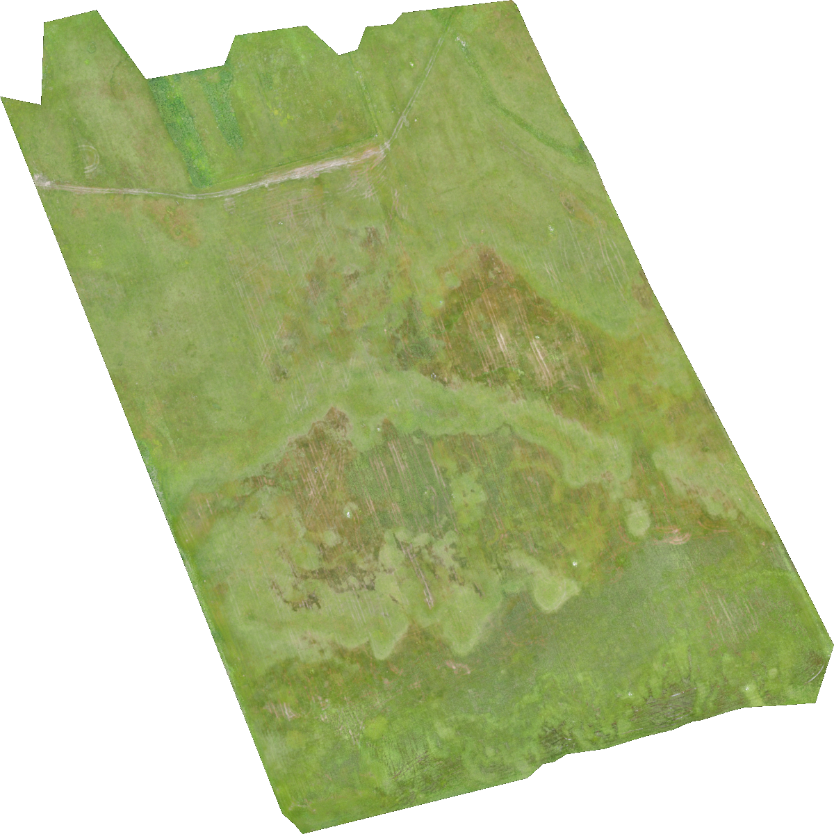
Every panel comes from a verified processed Saardu project raster. Select a product to compare what changes when the measurement domain, spectral band or derivation changes over the same survey footprint.
FORMULA / SOURCES.O.D.A. RGB orthomosaic
BANDS / DOMAINVisible Red + Green + Blue channels
WHAT YOU ARE SEEINGThe processed visible-light orthomosaic for the same Saardu survey footprint.
WHY IT LOOKS DIFFERENTThe source RGB colour rendering is retained and resampled to the common teaching grid; it is not a single reflectance band.
WHAT THE PIXELS REPRESENTDisplayed red, green and blue channel values in the processed orthomosaic.
WHAT WE CAN INFERVisible spatial context, boundaries and texture after geometric QA.
WHAT WE CANNOT INFERQuantitative surface reflectance, a plant trait or species identity from colour alone.
Same footprint: image, bands and derived products
Supporting science · open when a step links here
Field Lab reference desk
The operational timeline is the spine of this lab. These concise chapters explain the science behind its decisions without interrupting the chronological workflow.
01Flight design and the fixed-wing decisionPlatform · altitude · overlap · GSD
A fixed-wing eBee X was appropriate for systematic coverage of spatially extensive meadow sites. A multirotor remains preferable for hovering, tight launch areas and fine local inspection; neither platform is universally superior.
- Efficient forward coverage
- Longer endurance potential
- Cannot hover
- Needs suitable launch/recovery space
- Hover and oblique views
- Tighter launch/landing
- Fine local positioning
- Usually less area per battery
| System | Payload | Altitude | Overlap | Output GSD | Purpose |
|---|---|---|---|---|---|
| Multispectral | Parrot Sequoia | 106–109 m AGL | 80% forward · 75% side | ≈10 cm/pixel | Green, Red, Red Edge and NIR reflectance products |
| RGB | senseFly Duet T · S.O.D.A. RGB | 119–125 m AGL | 85–88% forward · 80–86% side | ≈2.7 cm/pixel | Visible context, texture, boundaries and photogrammetric geometry |
| Thermal | senseFly Duet T · 640 × 512 thermal | Project mission record | Paired Duet T acquisition | ≈15.6 cm/pixel | Thermal infrared product; not reflectance |
- 01Define survey boundary
Include the target meadow, required plots and operational margin; identify obstacles and an approved fixed-wing recovery area.
- 02Choose sensor
Choose RGB, Sequoia or Duet T from the required measurement domain—not from convenience alone.
- 03Choose required GSD
Relate research detail to nominal GSD, altitude, camera footprint, coverage and practical endurance.
- 04Set overlap
Set forward and side overlap so consecutive images and adjacent flight lines share enough stable content for reconstruction.
- 05Choose landing approach
Evaluate the landing direction and area under the current approved eBee procedure; this tutorial does not replace manufacturer training.
- 06Plan GCP distribution
Where control is used, distribute visible surveyed targets around and within the block; avoid one corner or a single line.
- 07Save and document
Record mission name, site, flight date, payload, planned GSD, altitude and both overlaps; capture the settings screen.
Pixel size is not always effective spatial resolution. Blur, motion, reconstruction, geolocation and resampling can reduce the detail that is scientifically distinguishable.
02What RGB, Sequoia and Duet T measureSpectrum · reflectance · thermal emission · indices
VISIBLERED EDGENIRTHERMAL INFRAREDGreenRedRed EdgeNIRDuet T thermal
Band explorer
Green
Visible green reflectance; useful context for vegetation colour and green–NIR contrasts. Pigments, illumination, canopy and background all contribute.
Project index
NDVI
(NIR − Red) / (NIR + Red)Why these bands: Red absorption contrasted with NIR scattering.
Project role: General vegetation-condition contrast.
Boundary: Can saturate; soil, canopy, atmosphere and shadows matter.
Visible colour and geometry
High-resolution visible imagery supports context, boundaries, texture and reconstruction. It is scientific evidence, not merely a normal picture.
Four reflectance bands
Green 550/40 nm, Red 660/40 nm, Red Edge 735/10 nm and NIR 790/40 nm are calibrated separately.
Thermal emission
S.O.D.A. RGB is paired with a 640 × 512 thermal camera. Thermal values represent emitted infrared/apparent surface temperature when calibrated—not reflectance.
THERMAL ≠ REFLECTANCETHERMAL ≠ DIRECT SOIL MOISTURETHERMAL ≠ DIRECT PLANT STRESS
RGB-derived points
thermal-looking palette
COLOUR PALETTE ≠ MEASUREMENT03Positioning and controlTime · RINEX · PPK · GCP · CRS
UAV GNSS
rover observations+Reference station
RINEX observations+Overlapping time
mission + margin→ PPK solution → corrected camera geotags
rover observations+Reference station
RINEX observations+Overlapping time
mission + margin→ PPK solution → corrected camera geotags
PPK combines rover and reference GNSS observations after flight. RINEX transfers receiver-independent observation/navigation data. In the documented 2024 project example, reported geotag uncertainty improved from approximately 0.806 m to 0.049 m; that is not a universal guarantee of map accuracy.
TIME CHECK
For the July 2024 mission, Estonia local time was UTC+3. Verify the source time basis and request reference data for the complete flight plus margin.
Where is this pixel?
- geotagging and PPK
- GCPs
- EPSG:3301
- bundle adjustment
- DSM and orthorectification
What does its value represent?
- sensor response
- illumination and calibration
- reflectance
- thermal signal
04What Pix4D reconstructsTie points · bundle adjustment · dense surface · orthorectification
Pix4D is not simply stitching pictures. Repeated features link overlapping views; bundle adjustment estimates camera geometry; dense reconstruction estimates the visible surface; the DSM then supports orthorectification into map geometry.
05Products, indices and failure boundariesRGB · DSM · reflectance · thermal · vegetation indices
| Product | Status | Pixel / sample meaning | Scale | Use | Limitation |
|---|---|---|---|---|---|
| RGB orthomosaic | processed | Orthorectified visible-colour mosaic | ≈2.7 cm/pixel | Context, boundaries, texture | Colour and texture are not species or trait measurements |
| Green reflectance | processed | Calibrated Green-band reflectance | ≈10 cm/pixel | Visible vegetation/background information | Illumination and calibration quality remain consequential |
| Red reflectance | processed | Calibrated Red-band reflectance | ≈10 cm/pixel | Pigment-sensitive contrast; NDVI input | Not a direct chlorophyll reading |
| Red Edge reflectance | processed | Calibrated Red Edge reflectance | ≈10 cm/pixel | Red-edge indices and modelling | Sensitive to registration and calibration |
| NIR reflectance | processed | Calibrated NIR reflectance | ≈10 cm/pixel | Canopy/leaf scattering and indices | Water, shadows and background can dominate |
| DSM | derived | Elevation of the visible upper surface | output-grid dependent | Surface structure and height-related predictors | DSM is not a bare-earth DEM |
| Point cloud | derived | 3-D reconstructed surface samples | irregular 3-D support | Geometry QA and DSM production | Density is not accuracy |
| Thermal product | processed | Thermal infrared signal / apparent surface temperature where calibrated | ≈15.6 cm/pixel | Surface-temperature pattern inspection | Not reflectance, soil moisture or plant stress directly |
| Vegetation indices | derived | Formula applied to compatible reflectance bands | aligned output grid | Compact spectral predictors | Band ≠ index; index ≠ trait |
BAND ≠ INDEXINDEX ≠ TRAITTRAIT PREDICTION ≠ DIRECT MEASUREMENT
(NIR − Red) / (NIR + Red)Why: Red absorption contrasted with NIR scattering.
Use: General vegetation-condition contrast.
Failure boundary: Can saturate; soil, canopy, atmosphere and shadows matter.
(NIR − Green) / (NIR + Green)Why: Green-to-NIR contrast.
Use: Complementary canopy and pigment-sensitive predictor.
Failure boundary: Does not directly measure chlorophyll or photosynthesis.
((NIR − Red) / (NIR + Red + 0.5)) × 1.5Why: Adds a documented soil-adjustment term.
Use: Sparse vegetation and exposed-background conditions.
Failure boundary: L = 0.5 is a parameter choice, not universal correction.
(2NIR + 1 − √((2NIR + 1)² − 8(NIR − Red))) / 2Why: Adaptive red–NIR soil adjustment.
Use: Complementary predictor where soil background is visible.
Failure boundary: Requires valid reflectance, masks and a non-negative radicand.
(NIR − Red) / √(NIR + Red)Why: Renormalizes the red–NIR contrast.
Use: Vegetation-density sensitivity in the project predictor set.
Failure boundary: Not NDVIRe; denominator and reflectance scale must be valid.
100(NIR − Red Edge) − 10(NIR − Green)Why: Combines NIR, Red Edge and Green contrasts.
Use: Red-edge-sensitive canopy/pigment predictor.
Failure boundary: Empirical relationship must be validated for this campaign.
NIR / Red EdgeWhy: NIR-to-Red Edge ratio.
Use: Canopy-condition and red-edge predictor.
Failure boundary: Unstable when the denominator is invalid or near zero.
(NIR / Red Edge) − 1Why: Shifted red-edge simple ratio.
Use: Chlorophyll-associated project predictor.
Failure boundary: An index, not a direct CCI or chlorophyll measurement.
HIGH NDVI ≠ HIGH BIODIVERSITYHIGH NDVI ≠ AUTOMATICALLY HIGH BIOMASSHIGH NDVI ≠ DIRECT CHLOROPHYLL
06From 1 m² plot to ecological modelSupport · aggregation · prediction · non-claims
CCI · leaf area · height · AGB/productivity · species and cover
Green · Red · Red Edge · NIR · indices · DSM
Fitted relationship → continuous prediction map
leafplant1 m² quadratmany UAV pixelsplot raster summaryprediction surface
Plot responses are paired with plot-level raster summaries. Treating every pixel inside a quadrat as an independent field observation manufactures replication and ignores biological support.
Continue through the Species Atlas field-to-EO evidence chain →Final failure gallery
A completed process can still be unusable
Portfolio challenge
Produce an auditable mission handoff
Evidence and software references