XGBoost from First Principles

1. Problem — XGBoost should not be a mysterious parameter dictionary

Learning outcome

By the end of this lesson, you will be able to explain XGBoost as a regularised additive tree model, connect objective, loss, gradient, Hessian, split gain, learning rate and sequential trees, predict the behavioural effect of its main parameters, describe its missing-value routing without treating missingness as solved, and identify when advanced categorical or structural constraints answer a real scientific need.

• Lesson type: XGBoost Mechanism Studio
• Estimated time: 190–260 minutes
• Prerequisites: Lessons 3.5–3.6; the target, predictor and experiment contracts from Chapter 1; Module 1 arrays and functions
• Portfolio output: xgboost_mechanism_notebook.ipynb

Why this matters

XGBoost is powerful enough to produce strong-looking results from a weak experiment. A learner can copy ten parameters, fit hundreds of trees and obtain a score without understanding what was optimised, why a split was accepted, how missing values were routed or which constraints shaped the function.

That is not defensible remote-sensing modelling. A scientist should be able to explain why the objective matches the target, how each tree changes the current prediction, which settings increase or restrict flexibility, and which evidence will later test generalisation.

Core lesson: XGBoost is an optimisation procedure for a declared predictive objective. It does not choose the scientific question, prevent leakage, define a transfer domain or turn feature importance into causality.

Mental model

Begin with a current prediction. Measure how the chosen loss would improve. Fit a tree whose leaves propose updates. Penalise unnecessary complexity. Scale the update by the learning rate. Add it to the model. Repeat.

current prediction
      ↓
loss gradients and curvature
      ↓
candidate split gains under regularisation
      ↓
new tree with leaf updates
      ↓ × learning rate
updated additive prediction

The model is the sum of all accepted tree contributions. The procedure is sequential because the next gradients depend on the current ensemble.

2. Scientific context — model the synthetic target, preserve the real limits

Use the same synthetic Chapter 2 data and frozen feature schema as Lessons 3.5–3.6. The objective is continuous regression for vegetation_height_cm. The teaching pack supplies this unit and definition; it does not transfer those meanings to undocumented fields in the published Baltic dataset.

Candidate predictors include EO-style indices, texture and a UAV height percentile. They may contain nonlinear predictive information. They remain proxies with support, timing and operational-availability constraints. A complex model can amplify a proxy’s usefulness and its failure modes at the same time.

The sealed final test rows remain unopened. This lesson studies mechanism with development evidence. Lesson 3.8 will fit one documented candidate; Chapter 3 will evaluate validation designs; Chapter 4 will tune only within the permitted development boundary.

3. Concept — objective equals loss plus regularisation

XGBoost describes learning through an objective containing two parts:

$$Objective = Training\ loss + Regularisation$$

For observations $(x_i,y_i)$ and an additive ensemble with $T$ trees:

$$\mathcal{L}^{(T)} = \sum_i l(y_i,\hat{y}_i^{(T)}) + \sum_{t=1}^{T}\Omega(f_t)$$

The loss states what predictive error means. For the Chapter 2 continuous target, squared error is a clear starting objective. Classification would require an objective such as logistic loss with a defined label and probability interpretation.

The regularisation term penalises model complexity. In XGBoost’s tree formulation it can penalise additional leaves and large leaf weights. This changes which split gains are worthwhile and how extreme an update becomes.

Regularisation does not guarantee ecological plausibility. It constrains the fitted function under the mathematical objective. A leaked predictor can still produce a strongly regularised but invalid model.

Check your understandingWhat does the XGBoost objective combine?

Choose one answer

Training loss and a regularisation termAccuracy and causal certaintyOnly the number of trees

Check answer

4. Additive learning and gradients

At boosting stage $t$, the prediction becomes:

$$\hat{y}_i^{(t)} = \hat{y}_i^{(t-1)} + \eta f_t(x_i)$$

where $f_t$ is the new tree and $\eta$ is the learning rate. XGBoost uses a second-order approximation of the loss around the current prediction. For each observation it calculates:

$$g_i = \frac{\partial l(y_i,\hat{y}_i)}{\partial \hat{y}_i} \qquad h_i = \frac{\partial^2 l(y_i,\hat{y}_i)}{\partial \hat{y}_i^2}$$

The gradient $g_i$ indicates the local direction and magnitude of loss change. The Hessian $h_i$ describes local curvature. Candidate leaves aggregate these values. The algorithm evaluates whether splitting one leaf into two improves the regularised objective enough to justify the extra structure.

A simplified split-gain form is:

$$Gain = \frac{1}{2}\left[ \frac{G_L^2}{H_L+\lambda}+ \frac{G_R^2}{H_R+\lambda}- \frac{(G_L+G_R)^2}{H_L+H_R+\lambda} \right]-\gamma$$

Here $G$ and $H$ sum gradients and Hessians in the candidate left and right leaves. $\lambda$ is L2 regularisation on leaf weights; $\gamma$ is the minimum loss reduction required for an added split in the tree-booster parameterisation.

You do not need to derive the optimiser. You do need to interpret the effects:

• larger reg_lambda shrinks leaf weights more strongly;
• larger gamma requires more gain before adding a split;
• insufficient child evidence can be restricted through min_child_weight;
• deeper trees can represent higher-order conditional partitions.

These controls act together. They are not independent quality sliders.

5. Visual explanation — sequential learning under one objective

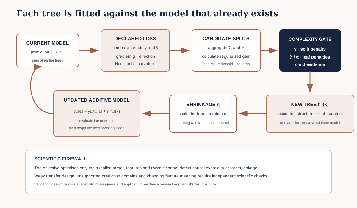
The diagram shows why tree order matters. Tree 2 is not another independent opinion about the original targets. It is selected after Tree 1 has changed the predictions. The regularisation gate is present at every stage; the learning rate scales every accepted contribution.

6. Worked example — make one additive update visible

Predict before running

The current model predicts 24 cm for four observations. A small tree proposes corrections of −4, −2, +3 and +5 cm. With a learning rate of 0.3, will the full corrections be added? Calculate the first and fourth updated predictions by hand.

import numpy as np

observed = np.array([19.0, 23.0, 29.0, 33.0])
prediction_0 = np.full(observed.shape, 24.0)
tree_1_correction = np.array([-4.0, -2.0, 3.0, 5.0])
learning_rate = 0.3

prediction_1 = prediction_0 + learning_rate * tree_1_correction
residual_0 = observed - prediction_0
residual_1 = observed - prediction_1

print("before:", prediction_0)
print("after: ", prediction_1)
print("squared error before:", np.sum(residual_0 ** 2))
print("squared error after: ", np.sum(residual_1 ** 2))

Code walkthrough

1. NumPy represents aligned observations and predictions.
2. observed supplies four instructional targets.
3. np.full(...) creates the initial constant prediction.
4. tree_1_correction stands for one fitted tree’s leaf outputs for these observations.
5. learning_rate=0.3 means only 30% of each proposed correction is added.
6. prediction_1 applies the additive update.
7. Residual arrays record target minus prediction before and after the update.
8. The final lines compare summed squared errors.

This example exposes shrinkage, not the XGBoost optimiser. In a fitted model, leaf corrections are learned from gradients, Hessians, candidate split gains and regularisation. Do not manually calculate and supply corrections during ordinary XGBoost training.

Diagnostic check

Assert that:

assert np.allclose(prediction_1, [22.8, 23.4, 24.9, 25.5])
assert np.sum(residual_1 ** 2) < np.sum(residual_0 ** 2)

Then try learning_rate=1.0 and 0.05 without changing the correction vector. Describe the size of one update, not final generalisation. A smaller step can still produce a worse complete model if the stage count, tree structure or objective is unsuitable.

Check your understandingWhat does a smaller learning rate do to each new tree's contribution?

Choose one answer

Shrinks it, usually requiring more boosting roundsDeletes all previous treesGuarantees generalisation

Check answer

7. Main parameters — explain effects, not recipes

Parameter	Mechanism	Increasing it tends to…	Scientific risk to inspect
n_estimators	number of boosting trees in the scikit-learn estimator	add more stages and capacity	training continues after validation improvement has ended
learning_rate	scales each tree contribution	make each stage more conservative, usually requiring more trees when decreased	copying a rate without coordinating tree count
max_depth	maximum tree depth	allow more conditional partitions and interactions	small samples support unstable high-order rules
min_child_weight	minimum summed instance weight/Hessian needed in a child	require more evidence before creating small child regions	rare but valid ecological conditions may be merged, or tiny artefacts may be fitted when too low
subsample	row fraction used for each boosting stage	introduce more row subsampling when below 1	structured sites may be represented unevenly; this is not a substitute for spatial validation
colsample_bytree	feature fraction sampled per tree	increase feature randomisation when below 1	important sensor groups may be omitted unpredictably without a schema-aware plan
gamma	minimum loss reduction for another split	demand stronger gain and reduce splitting	a numeric threshold is mistaken for scientific importance
reg_alpha	L1 penalty on leaf weights	favour more strongly shrunk or zeroed leaf weights	sparse behaviour is described as feature selection without evidence
reg_lambda	L2 penalty on leaf weights	shrink leaf updates more smoothly	regularisation is treated as protection from leakage or domain shift

Parameter effects are conditional. For example, reducing learning rate while leaving too few estimators can underfit. Raising depth while raising child-weight and regularisation may not behave like depth alone. Chapter 4 will define search spaces and learning diagnostics; Chapter 2 records one conservative starting configuration without optimisation.

8. Missing values — algorithmic routing is not scientific resolution

For tree boosters, XGBoost can represent missing numerical values and learn a default branch direction for a split from training evidence. When an observation lacks that feature at prediction time, it follows the learned default direction.

This is useful, but it answers only “how does the model compute a prediction?” It does not answer:

• Why is the value missing?
• Does missingness differ by site, sensor, habitat or season?
• Will the same missing-value representation be used operationally?
• Is an absent band a quality failure that should block prediction?
• Is missingness itself indirectly revealing the target or acquisition campaign?

Never replace a structural “not applicable” state with a numeric zero unless zero has that documented meaning. Preserve missingness profiles by split and domain. Compare training and prediction-time missingness. If a required sensor fails, the correct action may be to withhold a prediction rather than follow a default branch.

Check your understandingXGBoost learns a default branch for missing feature values. What must the scientist still check?

Choose one answer

Whether missingness has the same meaning and frequency during predictionNothing; automatic handling makes missingness scientifically harmlessOnly whether the CSV opens

Check answer

9. Classification counterpart

XGBClassifier uses the same additive tree logic but a classification objective changes what the raw score and transformed output represent. For binary classification, a logistic objective can return positive-class probabilities. The label definition, positive class, imbalance, probability evaluation and decision threshold must be declared.

Do not transfer regression metrics directly. Do not call a probability a class until a threshold and decision policy are specified. Lesson 3.16 will examine threshold choice and rare habitats; Lesson 3.18 will evaluate probability calibration and classification performance.

The model family does not define the problem type. The target contract does.

10. Optional advanced lab — constraints with a scientific reason

These capabilities remain optional. They are not extra badges and should be used only when the scientific and operational contract justifies them.

Native categorical support

Current XGBoost supports categorical features through documented DataFrame category types and enable_categorical=True with compatible tree methods and serialization. A scientist might need this when a genuinely nominal acquisition or environmental category is operationally available and one-hot encoding would be unwieldy.

Before using it:

• define category meanings and allowed levels;
• decide how unseen categories are handled;
• preserve category codes and model format;
• validate transfer across groups;
• avoid treating arbitrary numeric codes as ordered measurements.

Monotonic constraints

A monotonic constraint restricts a feature’s fitted direction. It can be useful when a relationship must obey a well-supported physical or operational rule over the declared domain. It is dangerous when ecology is nonlinear, proxies change meaning or interactions reverse local relationships.

Record the evidence for every constraint and compare constrained and unconstrained validation behaviour. A plausible-looking constraint is not proof of mechanism.

Interaction constraints

Interaction constraints restrict which feature groups may interact in trees. They can encode measurement-system boundaries, reduce implausible combinations or improve governance. They can also suppress real predictive structure if chosen from intuition alone.

Why would a scientist need these?

Use an advanced feature when it makes the predictive contract more faithful, reproducible or operational—not merely because the API exposes it.

11. Model clinic — copied parameters with no experiment history

Situation: a notebook declares max_depth=12, learning_rate=0.01, n_estimators=3000, subsample=0.8 and several penalties because a public notebook used them for another dataset.

Question	Diagnosis
problem	parameters have no connection to this target, sample, metric, validation or compute budget
evidence	no parameter-effect hypotheses, starting configuration, learning history or development-only search record
consequence	the result cannot show whether complexity was necessary or selected without test influence
fix	return to a documented conservative candidate, explain each effect, and defer search to the controlled Chapter 4 design

The copied configuration may execute. Execution is not methodological justification.

12. Common mistakes and recovery

Calling every residual correction “the gradient”

• Why it happens: squared-error intuition is memorable.
• How to detect it: the explanation ignores objective-specific derivatives and Hessians.
• How to prevent it: label residual correction as an introductory squared-error picture; state the general derivative formulation.
• Consequence: classification and custom objectives are misunderstood.

Treating more trees as independent replication

• Why it happens: the ensemble contains many components.
• How to detect it: uncertainty or sample size is calculated from tree count.
• How to prevent it: keep observation evidence distinct from model components.
• Consequence: confidence is overstated.

Assuming regularisation prevents leakage

• Why it happens: penalties are associated with generalisation.
• How to detect it: leaked target-derived predictors remain in the schema.
• How to prevent it: enforce Chapter 1 predictor and split contracts before fitting.
• Consequence: an invalid signal is efficiently learned.

Allowing missingness patterns to change silently

• Why it happens: XGBoost accepts NaN without imputation.
• How to detect it: missing rates differ sharply between training and operational data.
• How to prevent it: version missingness profiles and define blocking QA rules.
• Consequence: default routes encode conditions absent from validation.

Explaining parameters as universal directions

• Why it happens: tables say “higher means more conservative” without context.
• How to detect it: combined effects and learning-rate/tree-count trade-offs are ignored.
• How to prevent it: vary one factor for mechanism study, then tune jointly inside development folds.
• Consequence: intuition becomes an unreliable recipe.

Interpreting gain as causality

• Why it happens: a split-gain formula appears to quantify importance.
• How to detect it: high gain becomes “the feature controls vegetation.”
• How to prevent it: reserve interpretation for Chapter 5 and maintain the predictive claim boundary.
• Consequence: model allocation of predictive credit is presented as ecological mechanism.

13. Guided practice — construct a parameter-effect notebook

1. Reproduce the manual additive update and verify it by hand.
2. Draw the objective as loss plus regularisation in Markdown.
3. Explain gradient and Hessian in your own words without deriving the optimiser.
4. Annotate the split-gain terms $G_L,H_L,G_R,H_R,\lambda,\gamma$.
5. Create a table for all nine core parameters with mechanism, expected effect and risk.
6. For learning rate, test several values on the fixed correction vector.
7. For a fitted toy model, inspect the first tree only; do not infer a final ecological rule.
8. Profile missingness by feature and split in the synthetic pack.
9. Write an operational response for missing predictor, failed sensor and out-of-domain feature.
10. Choose one optional advanced constraint and state a situation where it would be justified and one where it would distort the problem.
11. Record XGBoost version, objective and model-format decision.

14. Independent challenge — review a proposed XGBoost configuration

You receive this proposal:

XGBRegressor(
    n_estimators=2000,
    learning_rate=0.01,
    max_depth=10,
    min_child_weight=1,
    subsample=0.6,
    colsample_bytree=0.5,
    gamma=0,
    reg_alpha=0,
    reg_lambda=1,
)

Do not decide whether it is “good.” Produce a review table with:

• intended effect of each setting;
• interaction with at least one other setting;
• evidence required to justify it;
• overfit or underfit risk;
• operational implication;
• whether the setting belongs in the initial candidate or later tuning.

Conclude with a simpler starting configuration and a Chapter 4 search hypothesis. Keep the final test outside the review.

15. Scientific interpretation

XGBoost can represent nonlinear, interacting predictive structure through a regularised sequence of trees. A strong result would mean that the fitted feature schema contains information useful for the target under the evaluated design. It would not prove that the predictors cause vegetation height, that fitted thresholds are ecological laws, or that the model is supported outside the training domain.

Understanding the objective makes failure easier to diagnose. A wrong target means the loss optimises the wrong quantity. Leakage means the loss rewards forbidden information. A weak split means the score measures the wrong transfer claim. Domain shift means future gradients were never represented in training.

The algorithm can optimise only the problem it receives. Scientific defensibility comes from the complete evidence chain.

16. Reflection, submission and portfolio artifact

Reflection

1. What two terms form the XGBoost objective?
2. Why does the next tree depend on the current ensemble?
3. How do learning rate and tree count interact?
4. What does gamma require from a candidate split?
5. Why is automatic missing-value routing not a missingness policy?
6. When could a monotonic constraint harm an ecological model?

Submission

Submit:

• xgboost_mechanism_notebook.ipynb;
• parameter_decision_record.csv;
• one annotated sequential-learning diagram;
• one missingness and operational-response table;
• a 450–650 word explanation of the objective, additive updates, main parameters and scientific limits.

Portfolio artifact

Artifact 3.7 — XGBoost Mechanism and Parameter Decision Record

This artifact demonstrates that you understand what the algorithm optimises and can defend a starting configuration before fitting the first candidate. It becomes the rationale attached to the serialized model in Lesson 3.8.

17. Core references and advanced reading

• XGBoost: Introduction to Boosted Trees
• XGBoost parameter reference
• XGBoost categorical data tutorial
• Chen and Guestrin (2016), XGBoost
• Friedman (2001), Greedy Function Approximation

Tested software versions

Python 3.12.13, NumPy 2.4.2, pandas 2.2.3, scikit-learn 1.9.0 and XGBoost 3.3.0. Parameter names and categorical-support guidance were checked against the stable XGBoost 3.3 documentation. Optional features must be rechecked against the learner’s installed version before use.