Train the First Defensible XGBoost Model

1. Problem — produce one model another scientist can inspect and reload

Learning outcome

By the end of this lesson, you will be able to fit one predeclared untuned XGBRegressor on the saved Chapter 2 development split, compare it with the established baseline on identical validation observations, preserve feature order and fold identity, serialize the model in JSON format, write complete sidecar metadata, reload it, reproduce predictions and explain why the result is a development candidate rather than final evidence.

• Lesson type: First Model Reproducibility Laboratory
• Estimated time: 210–280 minutes
• Prerequisites: Lessons 3.1–3.7 and their cumulative contracts; Module 1 reproducible notebooks and version records; Module 2 analysis-ready EO feature schemas
• Portfolio outputs: model.json, MODEL_METADATA.json, validation_predictions.csv, first_model_report.md

Why this matters

A model that exists only in notebook memory is not a professional artifact. A model file without its target, feature schema, data version, validation design and package versions is also incomplete. Future inference can fail silently if columns are reordered, transformations change or a predictor acquires a new meaning.

This lesson joins method and handover. The candidate must be traceable from the frozen experiment plan through training rows, fixed feature order, declared parameters, validation predictions, baseline comparison and serialized artifact. Another scientist should be able to answer: what was fitted, on which evidence, for which claim, using which software, and how do we know the saved file reproduces the model’s behaviour?

Core lesson: the first defensible model is not the most optimised model. It is the first candidate whose evidence, configuration, output and limitations can be independently reviewed.

Mental model

Treat the model as one component in an evidence package:

frozen experiment plan
        ↓
versioned data + saved split + ordered feature schema
        ↓
training-only fit
        ↓
baseline and XGBoost predictions on identical validation IDs
        ↓
metrics + diagnostics + limitations
        ↓
model.json + MODEL_METADATA.json + reload verification

If any arrow is missing, the model cannot be reconstructed or its performance claim cannot be interpreted.

2. Scientific context — the first Environmental Monitoring Project candidate

The target remains the synthetic vegetation_height_cm teaching response. Use the operational predictors approved in Lesson 3.3 and present in the Chapter 2 fixture:

1. sentinel2_ndvi;
2. sentinel2_ndmi;
3. uav_height_p95;
4. texture_contrast;
5. acquisition_gap_days only if the predictor register declares its measurement and availability as appropriate.

The exact feature list must match the frozen experiment plan. Do not add a feature because a correlation or trial run looks promising. Record an amendment if the plan genuinely changes; do not rewrite history.

Use chapter2_split=train for fitting and chapter2_split=validation for the instructional comparison. Do not load target summaries for sealed rows. Chapter 3 will ask whether the fixed split represents within-site, new-site or new-region generalisation. This limitation must appear in the report title or scope, not in small print.

3. Concept — one untuned candidate

The model is untuned because Chapter 2 has a different learning objective from Chapter 4. Here you will prove that the entire fit–predict–evaluate–save–reload chain is explicit. Tuning now would combine mechanism, search and evaluation before the validation architecture has been taught.

The starting configuration should be:

• specified before the fit;
• conservative enough to inspect;
• fully explained using Lesson 3.7 parameter effects;
• stable under a recorded seed;
• trained with controlled threading when exact reproducibility matters;
• unchanged after validation performance is viewed.

If performance is weak, preserve it. Weak evidence is a result. It can motivate a future hypothesis, but it does not authorise repeated hidden adjustments on the same validation set.

Check your understandingWhy is the first Chapter 2 XGBoost candidate intentionally untuned?

Choose one answer

To isolate a declared starting configuration before Chapter 3 validation and Chapter 4 tuningBecause XGBoost parameters never matterTo allow the final test set to choose settings

Check answer

4. Visual explanation — the first-model evidence chain

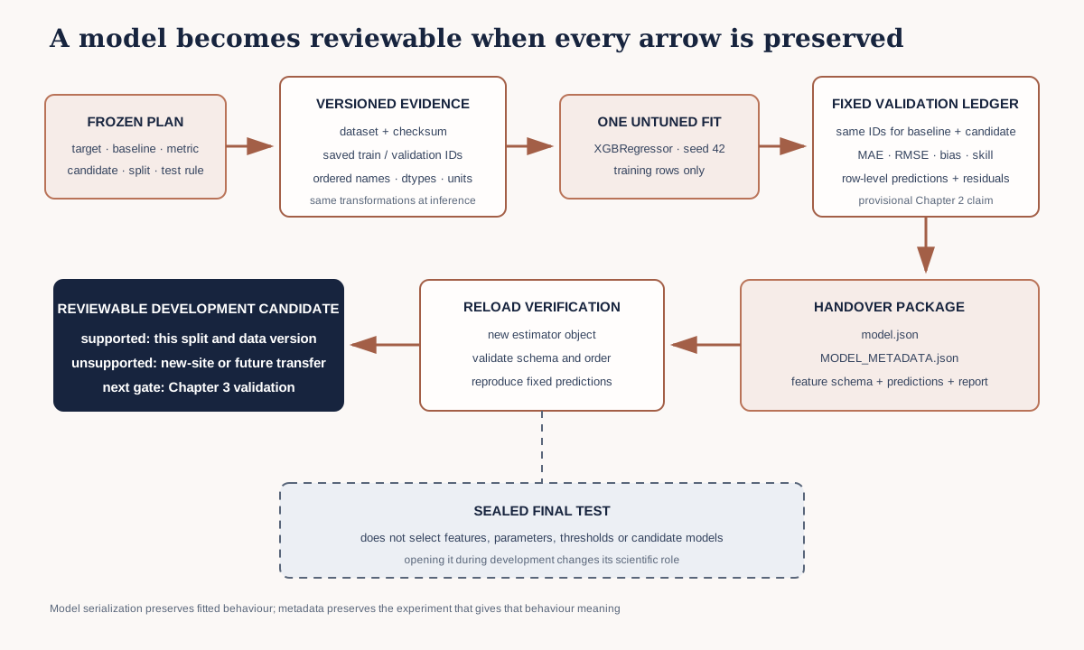
The diagram deliberately shows model.json and MODEL_METADATA.json as separate linked files. The serialized model preserves the fitted booster. The sidecar preserves experiment information that cannot be assumed to live inside the model artifact, including dataset and fold versions, intended use and unsupported claims.

5. Prepare the feature and split contract

Before importing XGBoost, print and save:

• dataset path, checksum and version;
• experiment-plan version;
• target specification version;
• predictor-hypothesis register version;
• fold-registry version;
• ordered feature names;
• expected dtypes and units;
• training and validation observation IDs;
• target unit;
• random seed;
• XGBoost and dependency versions.

Then validate:

feature names in data = frozen feature names
feature order used for fit = feature order used for predict
training IDs ∩ validation IDs = empty
training IDs ∩ sealed IDs = empty
validation IDs ∩ sealed IDs = empty
target missing among fit/score rows = zero
non-finite feature policy = documented

Equal column count is not enough. Two five-column tables can carry different meanings or order. Save a schema table with name, dtype, unit, transformation, source and missing_value_policy.

Check your understandingWhy record feature order even when a model file is saved?

Choose one answer

Inference must reproduce the same feature meanings, names, order and transformationsFeature order affects only plot coloursA JSON model stores the complete data provenance automatically

Check answer

6. Worked example — fit the declared XGBoost candidate

Predict before running

Review the Lesson 3.5 baseline MAE. Predict three possible outcomes: the candidate improves, matches or underperforms. For each, write the appropriate scientific response. Do not write a plan that changes parameters solely when the result disappoints.

import pandas as pd
from sklearn.metrics import mean_absolute_error
from xgboost import XGBRegressor

data = pd.read_csv("data/baseline_modelling_data.csv")
train = data.loc[data["chapter2_split"] == "train"]
validation = data.loc[data["chapter2_split"] == "validation"]
feature_order = ["sentinel2_ndvi", "sentinel2_ndmi",
                 "uav_height_p95", "texture_contrast"]

model = XGBRegressor(objective="reg:squarederror", n_estimators=200,
    learning_rate=0.05, max_depth=3, min_child_weight=3,
    subsample=0.8, colsample_bytree=0.8, reg_lambda=1.0,
    random_state=42, n_jobs=1)
model.fit(train[feature_order], train["vegetation_height_cm"])
predictions = model.predict(validation[feature_order])
print(mean_absolute_error(validation["vegetation_height_cm"], predictions))

Code walkthrough

1. pandas loads the versioned fixture.
2. MAE applies the primary baseline-comparison metric in centimetres.
3. XGBRegressor exposes XGBoost through a scikit-learn-compatible estimator.
4. Training and validation rows come from the saved split, not a new random call.
5. feature_order is a list because sequence is part of the inference contract.
6. objective="reg:squarederror" matches a continuous numerical target and squared-error training objective.
7. n_estimators=200 fixes the number of boosting stages for this starting candidate.
8. learning_rate=0.05 shrinks each tree contribution.
9. max_depth=3 limits conditional partition depth.
10. min_child_weight=3 requires a minimum amount of training weight/Hessian in a child.
11. Row and feature subsampling introduce controlled stochastic diversity.
12. reg_lambda=1.0 applies L2 regularisation to leaf weights.
13. random_state=42 records the estimator seed.
14. n_jobs=1 reduces parallel nondeterminism and oversubscription for this small reproducibility exercise; it is not a universal production requirement.
15. .fit(...) receives only the ordered development features and training target.
16. .predict(...) uses exactly the same ordered feature schema on validation rows.
17. The final line reports MAE but does not yet compare it, attach units or save row-level evidence. Add those steps in guided practice.

This configuration is a documented teaching start, not an Academy recommendation for every EO dataset. Do not change it after viewing the Chapter 2 validation score.

Diagnostic check

Before calculating a headline metric, confirm that the prediction vector has the same length and observation order as the validation registry, contains only finite values and was produced from the frozen feature sequence. Export the row-level ledger and compare its ID checksum with the baseline ledger. If any ID or order differs, stop the comparison rather than aligning values by position from memory.

7. Evaluate against the established baseline

Create validation_predictions.csv with:

observation_id
site
spatial_block
observed_vegetation_height_cm
mean_baseline_prediction_cm
linear_baseline_prediction_cm
xgboost_prediction_cm
xgboost_residual_cm
split_version
model_version

All prediction columns must align to the same ordered observation IDs. Calculate:

• baseline MAE and RMSE;
• XGBoost MAE and RMSE;
• MAE and RMSE skill relative to the declared baseline;
• mean signed residual as an early bias diagnostic;
• training versus validation errors;
• observed and predicted ranges.

Report a difference without overselling it. “The untuned candidate improved MAE by 2.1 cm on these fixed validation cases” is bounded. “XGBoost solves vegetation-height prediction” is unsupported.

If the candidate underperforms, keep the model artifact and write a failure note. Ask whether the feature set lacks information, the target is noisy, the configuration underfits, the validation domain differs, or the baseline already captures the relationship. Do not diagnose from one metric alone.

8. Model metadata — the model file is not the experiment

Write MODEL_METADATA.json containing:

{
  "model_version": "m3-ch2-xgbreg-001",
  "model_family": "XGBRegressor",
  "objective": "reg:squarederror",
  "target_specification_version": "...",
  "dataset_version": "...",
  "dataset_sha256": "...",
  "fold_registry_version": "...",
  "feature_order": ["..."],
  "feature_schema_path": "feature_schema.csv",
  "parameters": {},
  "random_seed": 42,
  "training_observation_count": 0,
  "validation_observation_count": 0,
  "validation_metrics": {},
  "software_versions": {},
  "final_test_opened": false,
  "intended_use": "...",
  "unsupported_use": "..."
}

Also record training timestamp, platform, training duration, output paths and a checksum for each artifact. Do not place secrets, machine usernames or inaccessible absolute paths in portfolio metadata.

XGBoost’s JSON or UBJSON model formats preserve the fitted model representation and feature names where supported. They do not replace the full data, validation and experiment record. Parameter and metric provenance should remain explicit in the sidecar.

9. Serialize, reload and verify

Save in JSON format:

model.save_model("models/model.json")

Then create a new estimator object, load the file and predict the fixed validation feature table:

import numpy as np
from xgboost import XGBRegressor

restored = XGBRegressor()
restored.load_model("models/model.json")
restored_predictions = restored.predict(validation[feature_order])
assert np.allclose(predictions, restored_predictions, rtol=0, atol=1e-10)

The strict tolerance is appropriate only if the same environment and deterministic path reproduce the model. If hardware, device or version changes produce small numerical differences, predeclare an evidence-based tolerance and verify that metrics and decisions remain stable. Never loosen a tolerance until a failing comparison passes without investigation.

Also test intentional failure:

• remove one feature;
• rename one feature;
• reorder the DataFrame columns;
• change one dtype.

Your schema validator should block these inputs before prediction or document exactly which estimator-level feature checks are relied upon. The safest inference interface explicitly selects and validates the recorded feature order.

Check your understandingWhat is the strongest save/load check?

Choose one answer

Reload the model and confirm predictions match on a fixed verification tableConfirm that model.json existsRename the file after fitting

Check answer

10. Reproducibility is more than a seed

A random seed controls some stochastic decisions. It does not preserve:

• row order;
• data values;
• library implementations;
• compiler and hardware behaviour;
• thread scheduling;
• feature transformations;
• fold assignments;
• target definitions.

For this exercise, record random_state, use the saved split and feature table, set n_jobs=1, preserve package versions and test saved predictions. Later production workflows may use parallel or GPU execution for justified scale. They should define acceptable numerical tolerance and decision stability rather than claiming bitwise identity across every platform.

Model reproducibility has levels:

1. artifact reproducibility — the saved model reloads;
2. prediction reproducibility — it reproduces predictions on a fixed verification table;
3. training reproducibility — the complete environment and evidence recreate an equivalent fitted model;
4. scientific reproducibility — another team can reconstruct the target, features, validation claim and interpretation.

Your portfolio package should support all four as far as the instructional evidence permits.

11. Classification counterpart — same workflow, different contract

For a categorical target, use XGBClassifier only after defining:

• class meanings and authoritative labels;
• positive class where relevant;
• rare-class prevalence;
• classification objective;
• probability versus class output;
• validation metrics;
• threshold policy;
• class-weight or sampling decisions;
• probability calibration plan.

The workflow remains experiment plan → saved folds → baseline → candidate → predictions → evaluation → diagnostics → serialization. The metrics and decision rules change. Do not use regression MAE for class labels, and do not accept default accuracy as sufficient.

This lesson introduces the counterpart but does not add a classification fit to the core submission. Lesson 3.16 will build the rare-habitat decision policy before the full classification evaluation in Lesson 3.18.

12. Model clinic — a saved model with no feature contract

Situation: a colleague sends model.json. It loads successfully, but the only accompanying table contains five unnamed columns. The production stack also has five columns, so the team proceeds.

Question	Diagnosis
problem	dimensional equality is mistaken for semantic equality
evidence needed	feature names, order, dtype, unit, transformation, acquisition rule and model metadata
consequence	valid-looking predictions may be assigned to the wrong measurements
fix	block inference until the versioned schema is restored and verify predictions on a known table

The correct response is not to guess from plausible output ranges. A wrong feature order can still generate finite values and a visually convincing map.

13. Common mistakes and recovery

Tuning after seeing the validation result

• Why it happens: the first candidate feels provisional.
• How to detect it: parameters change without a predeclared search record.
• How to prevent it: freeze the candidate and preserve amendments; tune later inside nested development logic.
• Consequence: the validation estimate becomes part of model selection.

Recreating the split with train_test_split

• Why it happens: tutorials commonly begin with a random split.
• How to detect it: saved observation-to-fold assignments are ignored.
• How to prevent it: join the immutable registry by observation ID.
• Consequence: comparisons no longer refer to the experiment plan.

Selecting columns through unordered structures

• Why it happens: feature membership is confused with feature sequence.
• How to detect it: fit and inference code derive columns differently.
• How to prevent it: store one ordered list and validate names, dtypes and transformations.
• Consequence: model inputs change meaning.

Saving only a pickle

• Why it happens: object serialization is convenient.
• How to detect it: no stable XGBoost model format or environment record exists.
• How to prevent it: use documented JSON/UBJSON model IO plus explicit metadata and environment files.
• Consequence: portability, security and long-term readability are weakened.

Reporting one score without row-level predictions

• Why it happens: a metric is compact.
• How to detect it: errors cannot be linked to sites, blocks or observations.
• How to prevent it: save a prediction ledger keyed by observation ID.
• Consequence: Chapter 3 validation and Chapter 5 diagnostics cannot audit failure.

Calling the validation result final performance

• Why it happens: the notebook completed successfully.
• How to detect it: no independent test or structured-transfer evaluation exists.
• How to prevent it: label the artifact “Chapter 2 development candidate.”
• Consequence: a preliminary comparison is overstated as operational evidence.

14. Guided practice — build the complete first-model package

1. Verify all Chapter 1 and Chapter 2 checksums.
2. Load the frozen experiment plan and confirm it names the baseline, metric, candidate and split.
3. Load the saved row registry by observation ID.
4. Validate feature names, order, dtypes, units and missingness policy.
5. Assert split disjointness without summarising sealed targets.
6. Reproduce mean and linear baseline predictions.
7. instantiate the declared XGBRegressor exactly once.
8. Fit using training rows only.
9. Predict the fixed validation rows in registry order.
10. Save row-level baseline and candidate predictions.
11. Calculate MAE, RMSE, bias and baseline skill.
12. Plot observed versus predicted and residual versus fitted values as preliminary diagnostics.
13. Save model.json and MODEL_METADATA.json.
14. Reload the model in a fresh object and compare predictions.
15. Run schema-failure tests.
16. Restart the notebook kernel and run all cells from top to bottom.
17. Write first_model_report.md with a limitation section naming the provisional validation claim.

15. Independent challenge — perform a handover without verbal explanation

Create a clean first_xgboost_model/ folder containing:

README.md
model.json
MODEL_METADATA.json
feature_schema.csv
validation_predictions.csv
validation_metrics.csv
baseline_scores.csv
first_model_report.md
environment.yml or equivalent lock record
checksums.sha256

Ask another person—or simulate a fresh project folder—to follow only the README. They must be able to:

1. identify intended and unsupported use;
2. load the model;
3. validate the supplied verification feature table;
4. reproduce saved predictions within the declared tolerance;
5. identify the validation design and why it is not yet final;
6. confirm the final test was not opened.

Record every ambiguity discovered and revise the documentation without changing the fitted model.

16. Scientific interpretation

If the XGBoost candidate improves over both constant and transparent baselines on the fixed Chapter 2 cases, it demonstrates additional predictive information under this development comparison. The improvement may arise from nonlinear thresholds, interactions or additive structure. It does not identify ecological causes.

The result is not yet a spatial-transfer estimate. Nearby or related observations may make the fixed split optimistic. Chapter 3 will compare random, grouped, spatial and temporal validation designs according to the intended claim. Chapter 4 will tune without using the final test. Chapter 5 will examine residual geography and interpretation; Chapter 6 will address uncertainty and applicability.

A serialized model is therefore a checkpoint, not a declaration of readiness. Its value is that the exact candidate and evidence can now be challenged rather than reconstructed from memory.

17. Reflection, submission and portfolio artifact

Reflection

1. Why was the candidate left untuned?
2. Which feature properties must future inference reproduce?
3. What information belongs in metadata rather than only model.json?
4. What does a matching reload prediction establish?
5. Why is a seed insufficient for scientific reproducibility?
6. Which validation claim remains unresolved?

Submission

Submit:

• the complete first_xgboost_model/ folder;
• the continuing Environmental Monitoring Project notebook;
• one screenshot of the successful reload verification;
• a 500–700 word first_model_report.md comparing baselines and candidate, stating the supported claim and naming the next validation requirement.

Portfolio artifact

Artifact 3.8 — First Defensible XGBoost Candidate

Together, Lessons 3.5–3.8 establish a comparator ladder, expose tree and boosting mechanisms, document XGBoost’s objective and parameters, and deliver a versioned model that can be reloaded and audited. Chapter 3 will now test whether its validation evidence matches the intended spatial and temporal generalisation claim.

18. Core references and advanced reading

• XGBoost Python package introduction
• XGBoost scikit-learn estimator interface
• XGBoost model IO
• scikit-learn common pitfalls
• The Turing Way: reproducible research

Tested software versions

Python 3.12.13, NumPy 2.4.2, pandas 2.2.3, scikit-learn 1.9.0 and XGBoost 3.3.0. Model IO uses XGBoost’s documented JSON format. Recheck compatibility, model-format guidance and reproducibility tolerances before using a different XGBoost version or hardware backend.