Trees, Ensembles and Boosting

1. Problem — understand what the ensemble is doing before trusting it

Learning outcome

By the end of this lesson, you will be able to trace an observation through a regression tree, explain split, threshold, node, leaf and depth, distinguish bagging and Random Forest averaging from sequential gradient boosting, compare their prediction behaviour on the same saved validation cases, and defend why no tree ensemble is universally superior.

• Lesson type: Tree and Ensemble Mechanism Laboratory
• Estimated time: 160–220 minutes
• Prerequisites: Lesson 3.5; Module 1 conditions, functions and arrays; Module 2 continuous EO predictors and analysis-ready feature tables
• Portfolio output: ensemble_reasoning.ipynb

Why this matters

Tree ensembles are widely used in Earth Observation because they can represent nonlinear relationships, thresholds and interactions without requiring every relationship to be written as an equation. That practical strength can encourage weak reasoning: import a classifier, copy a parameter dictionary, report a score and describe the model as intelligent.

A remote-sensing scientist needs a clearer account. What regions of feature space did the model create? What value does a leaf return? Why does averaging many randomized trees behave differently from adding trees sequentially? Which behaviour is useful for the target, sample size and transfer claim?

Core lesson: a tree ensemble is a defined prediction mechanism, not a scientific explanation and not a substitute for validation.

Mental model

A single tree asks a sequence of yes/no questions about predictor values. The answers route an observation to one leaf. An ensemble combines many such trees in one of two broad ways:

• parallel diversification and averaging — trees are made different, then their predictions are aggregated;
• sequential correction — each added tree improves the prediction produced by the current ensemble under a chosen loss.

Random Forest is the first pattern. Gradient boosting is the second. Both use trees; their learning logic is different.

2. Scientific context — thresholds in coastal-meadow predictors

The Chapter 2 synthetic training pack pairs a documented synthetic vegetation-height target with EO-style predictors. A shallow regression tree might split on uav_height_p95, separating lower and taller canopy structures. A later branch might separate observations using sentinel2_ndmi, which can act as a proxy for moisture-related spectral behaviour.

These splits are predictive partitions. They do not prove that a threshold is an ecological law. The chosen cut depends on the supplied sample, other predictors, the loss, depth constraints and validation design. A split on NDMI may capture vegetation moisture, management, soil background, acquisition conditions or correlated structure. Preserve the measurement hypotheses from Lesson 3.3.

Use only rows labelled train and validation. The sealed rows remain outside every comparison. Chapter 3 will later replace the instructional split with validation designs matched to spatial and temporal transfer claims.

3. Concept — one decision tree

Split and threshold

A split divides observations according to a rule such as:

uav_height_p95 <= 34.5 cm?

The predictor is uav_height_p95; 34.5 is the threshold. Observations satisfying the rule move left; the others move right. For regression with squared-error criteria, a candidate split is valuable when the resulting groups are more internally similar in target values than the unsplit node.

Node, leaf and depth

A node is a location in the tree. The first decision is the root node. An internal node contains another split. A leaf ends a path and returns a prediction. In a standard regression tree, that prediction is commonly the mean target of training observations reaching the leaf under the fitted criterion.

Depth is the number of split levels along a path. A depth-one tree, often called a stump, can divide the feature space once. Greater depth allows more specific partitions and interactions, but can also make predictions sensitive to small training differences.

Recursive partitioning

After the first split, the algorithm considers dividing each resulting region again. This recursion produces rectangular regions in predictor space. Each region receives a constant leaf value. A tree is therefore nonlinear while producing piecewise-constant predictions.

Suppose a fitted tree uses:

1. uav_height_p95 <= 34.5;
2. within the taller branch, sentinel2_ndmi <= 0.31.

An observation with UAV height percentile 39 cm and NDMI 0.28 follows right, then left, and receives the value in that leaf. The route is inspectable. Its scientific meaning remains conditional on the training evidence.

Check your understandingWhat does a regression-tree leaf store for prediction?

Choose one answer

A fitted output value for observations reaching that leafA causal explanation of the targetA new field measurement

Check answer

4. Visual explanation — from a partition to two ensemble strategies

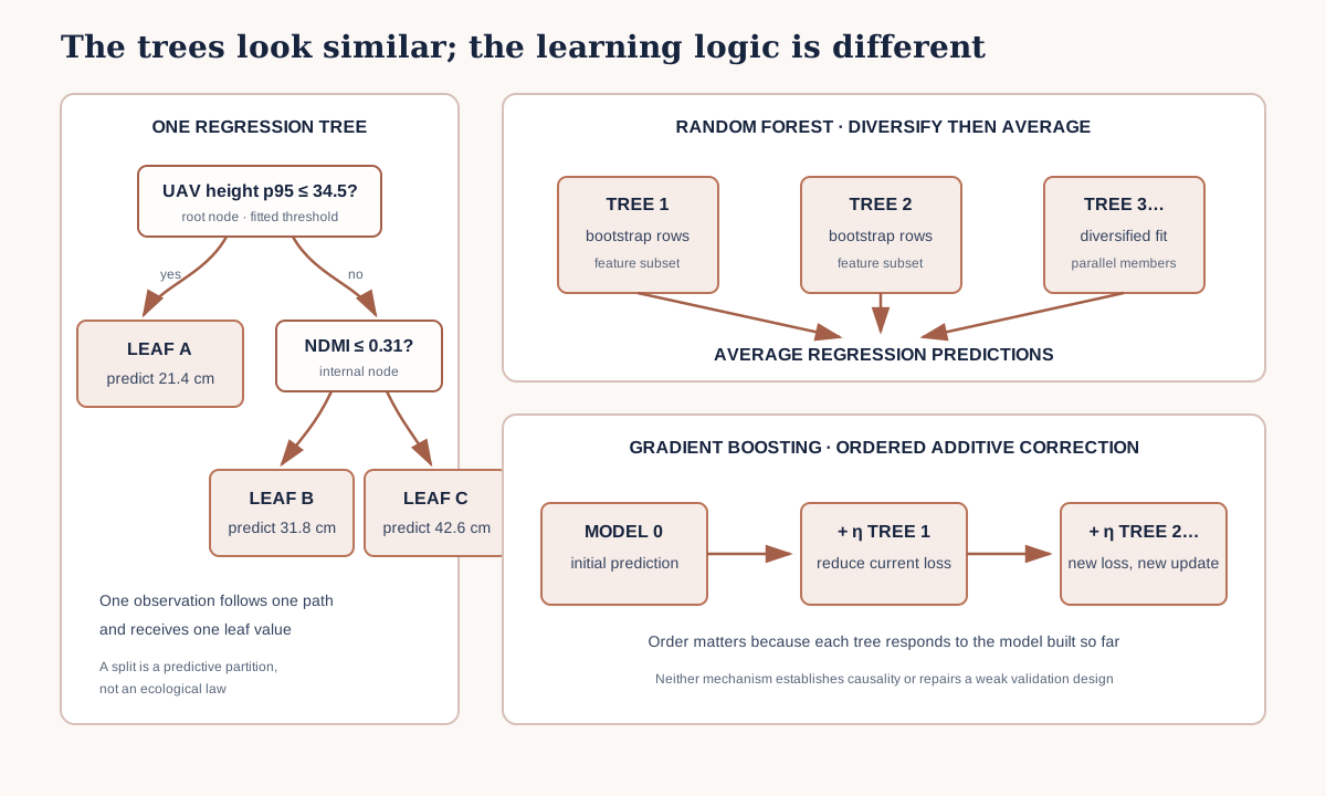
Read the figure from left to right. The single-tree panel shows routing. The upper ensemble branch shows several trees trained with randomisation and aggregated. The lower branch shows an evolving additive model: the next tree is selected in response to the current loss, not trained as an independent vote.

5. Bagging and Random Forest

Bagging

Bootstrap aggregating, or bagging, fits many versions of a base learner to resampled training data and averages their regression predictions or aggregates class predictions. A deep decision tree can have high variance: small data changes may alter early splits. Averaging diversified trees can reduce that instability.

The bootstrap samples are not new independent ecological observations. They are resamples of the available training evidence. Bagging changes the estimator; it does not expand the surveyed domain.

Random Forest

A Random Forest adds predictor randomisation. At candidate splits, each tree considers a random subset of features. This encourages diversity so that a few strong correlated predictors do not force every tree into the same structure.

For regression, the forest prediction is the average of tree predictions. Averaging can smooth individual-tree jumps, but the ensemble remains a function of learned partitions. It cannot safely extrapolate a continuous trend beyond represented predictor conditions merely because many trees agree.

Important controls include:

• number of trees;
• tree depth or minimum leaf size;
• number of predictors considered at each split;
• bootstrap sampling;
• random seed and parallel execution settings.

Do not tune them in this lesson. Use a documented comparison configuration to understand behaviour. Chapter 4 will introduce controlled optimisation.

6. Gradient boosting

Gradient boosting begins with a simple prediction and builds an additive model. Each new tree is selected to reduce the loss of the current ensemble.

For squared-error regression, a useful introductory picture is residual correction:

Model 0: initial constant prediction
       ↓ calculate remaining errors
Tree 1: model a correction
       ↓ update predictions
Tree 2: model the new remaining correction
       ↓
Tree 3: continue under the loss and constraints

Real gradient boosting is expressed through gradients of the chosen loss. XGBoost additionally uses second-order information and regularisation. Lesson 3.7 will establish those details. The residual picture is accurate intuition for squared error, not a universal algorithm description for every objective.

The ensemble prediction after $T$ stages can be written:

$$\hat{y}^{(T)}(x)=\hat{y}^{(0)} + \eta\sum_{t=1}^{T}f_t(x)$$

where $f_t$ is a fitted tree contribution and $\eta$ is the learning rate or shrinkage. Trees are not averaged as interchangeable independent members. Order matters because each tree is fitted relative to the model built so far.

Check your understandingWhat primarily distinguishes a Random Forest from gradient boosting?

Choose one answer

Forest trees are diversified and averaged; boosting trees are added sequentially to improve the current modelOnly a Random Forest uses treesBoosting never uses previous model error

Check answer

7. Worked example — expose the first split

Predict before running

Inspect the training scatterplot of uav_height_p95 against vegetation_height_cm. Predict approximately where a one-split tree will divide the feature. Which two mean leaf values do you expect? Record the prediction before fitting.

import pandas as pd
from sklearn.metrics import mean_absolute_error
from sklearn.tree import DecisionTreeRegressor

data = pd.read_csv("data/baseline_modelling_data.csv")
train = data.loc[data["chapter2_split"] == "train"]
validation = data.loc[data["chapter2_split"] == "validation"]
feature = ["uav_height_p95"]

stump = DecisionTreeRegressor(max_depth=1, random_state=42)
stump.fit(train[feature], train["vegetation_height_cm"])
predictions = stump.predict(validation[feature])

print(f"threshold: {stump.tree_.threshold[0]:.2f} cm")
print(f"validation MAE: {mean_absolute_error(validation['vegetation_height_cm'], predictions):.2f} cm")

Code walkthrough

1. pandas loads the same versioned Chapter 2 fixture used by the baseline report.
2. MAE preserves the target unit and supports the declared comparison.
3. DecisionTreeRegressor creates a continuous-target tree.
4. The saved split labels define fitting and scoring rows.
5. The one-feature list preserves DataFrame shape and feature name.
6. max_depth=1 restricts the tree to one split, making the mechanism inspectable.
7. random_state=42 records stochastic behaviour where applicable. A seed supports reproducibility but does not validate the split.
8. .fit(...) learns the threshold and two leaf values from training evidence.
9. .predict(...) routes validation observations through the learned rule.
10. tree_.threshold[0] exposes the fitted root threshold. The underscore marks a fitted attribute in scikit-learn conventions.
11. MAE evaluates exactly the validation targets used for the baseline ladder.

Diagnostic check

Export a table containing observation_id, the predictor, observed target, predicted leaf value and residual. Sort by the predictor and confirm that only two unique predictions occur. Locate observations immediately below and above the threshold. A tiny predictor difference may cause a jump because the stump creates discrete regions.

This is not a defect by itself; it is the mechanism. The question is whether additional trees, averaging or sequential correction improve credible validation performance without hiding instability.

8. Compare one tree, a forest and gradient boosting

Fit three fixed configurations:

• a shallow DecisionTreeRegressor;
• a RandomForestRegressor with a documented number of trees and minimum leaf size;
• a GradientBoostingRegressor with a documented learning rate, tree depth and number of stages.

Use the same feature order, train rows, validation rows and metric functions. Do not report only the winner. Record:

• training and validation MAE;
• validation RMSE;
• number and identity of scoring observations;
• range and number of unique predictions;
• random seed;
• configuration;
• runtime;
• one observed-versus-predicted figure.

Interpret patterns rather than ranking names. A single tree may underfit. A forest may reduce tree instability. Boosting may capture additive corrections efficiently but may also become sensitive to stage count, learning rate and depth. Chapter 4 will study those learning dynamics.

9. Random Forest versus Gradient Boosting

Question	Random Forest	Gradient Boosting
How are trees related?	diversified members fitted for aggregation	ordered additions to the current model
Main combination	average or vote	sum of scaled tree contributions
Primary intuition	reduce variance through averaging	reduce loss through sequential correction
Typical tree role	individual trees can be relatively deep	individual trees are often weak/shallow additions
Sensitivity	depth, leaf size, feature subsampling, bootstrap and sample size	learning rate, stage count, depth, regularisation and loss
Does it prove mechanism?	no	no
Universal winner?	no	no

“Random Forest is robust” and “boosting is more accurate” are not scientific conclusions. Define the data regime, metric, validation claim and uncertainty before comparing them.

Check your understandingWhen is Gradient Boosting universally superior to Random Forest?

Choose one answer

Never; performance and operational suitability must be evaluated for the stated problemWhenever the dataset contains EO predictorsWhenever more than one tree is fitted

Check answer

10. Model clinic — the forest that memorises field structure

Situation: a Random Forest has almost zero training error and a low error on a random row split. Repeated measurements from the same plots appear in both sets.

Question	Diagnosis
problem	related observations cross the evaluation boundary
evidence	compare plot, site, date and spatial-block identities across fit and score rows
consequence	flexible partitions can recognise local structure rather than transfer to genuinely new plots or sites
fix	preserve the result as an instructional comparison, then evaluate the intended transfer claim with grouped or spatial folds in Chapter 3

Changing from Random Forest to boosting does not repair the validation design. Validation is part of the claim, not a property supplied by an algorithm name.

11. Common mistakes and recovery

Reading a split as an ecological threshold

• Why it happens: a precise threshold resembles a field rule.
• How to detect it: the report says vegetation changes because NDMI crosses the fitted value.
• How to prevent it: call it a sample- and objective-dependent predictive partition.
• Consequence: a model artefact is presented as mechanism.

Assuming more depth means more knowledge

• Why it happens: deeper trees represent more combinations.
• How to detect it: training error falls while validation error or stability worsens.
• How to prevent it: treat depth as capacity requiring controlled validation.
• Consequence: small sample peculiarities become rules.

Describing bootstrap rows as new data

• Why it happens: each tree sees a different resample.
• How to detect it: the effective evidence count is confused with tree count times row count.
• How to prevent it: retain original observation identities and survey-domain limits.
• Consequence: confidence and domain coverage are overstated.

Claiming every tree independently corrects residuals

• Why it happens: forest and boosting diagrams both show multiple trees.
• How to detect it: Random Forest is described as sequential boosting.
• How to prevent it: state whether trees are aggregated peers or ordered updates.
• Consequence: parameter effects and diagnostics are misunderstood.

Comparing different split or feature versions

• Why it happens: notebooks evolve between models.
• How to detect it: row hashes or feature order differ across score files.
• How to prevent it: load one immutable comparison registry and schema.
• Consequence: apparent algorithm differences include data differences.

Calling agreement uncertainty

• Why it happens: variation among forest trees is easy to calculate.
• How to detect it: tree spread is labelled a calibrated prediction interval without coverage testing.
• How to prevent it: reserve interval claims for Chapter 6 methods and empirical coverage checks.
• Consequence: an internal ensemble statistic is misrepresented as uncertainty evidence.

12. Guided practice — trace, compare and explain

1. Reproduce the training-mean baseline from Lesson 3.5.
2. Fit the one-split regression tree and export its threshold and leaf values.
3. Draw the tree using plain decision text or scikit-learn plotting tools.
4. Manually route three validation observations through the threshold.
5. Confirm the manual leaf predictions match .predict().
6. Fit the fixed shallow tree, Random Forest and Gradient Boosting comparison configurations.
7. Score identical validation IDs with MAE and RMSE.
8. Calculate error skill relative to the mean baseline.
9. Compare training and validation errors without declaring a final winner.
10. Change only one observation: note how a near-threshold value is routed, but do not edit source data.
11. Write one paragraph distinguishing averaging from sequential correction.
12. Record which mechanism you expect XGBoost to extend and why.

13. Independent challenge — build an ensemble mechanism audit

Choose one validation observation and create a three-panel audit:

1. single tree: list each threshold decision and final leaf value;
2. Random Forest: show predictions from five selected trees and their average;
3. Gradient Boosting: show the initial prediction and the first three scaled tree contributions.

Do not present selected trees as the complete model. Label them as an explanatory subset. Then answer:

• Which mechanism produced averaging?
• Which produced an ordered sum?
• Which prediction changed most if one component changed?
• Which scientific claim is supported by this trace?
• Which claims still require Chapter 3 validation and Chapter 6 uncertainty work?

14. Scientific interpretation

A decision tree converts continuous predictor space into fitted regions. That can be useful when vegetation response is nonlinear or predictors interact. A Random Forest stabilises many randomized partitions through aggregation. Gradient boosting builds a sequence focused on improving the current objective.

These mechanisms can exploit EO information, but they inherit the target definition, predictor limitations, sampling design and domain boundaries established in Chapter 1. A forest cannot convert an undocumented target into a valid measurement. Boosting cannot make a training-time-only predictor operational. Neither can make a random row split support a new-region claim.

The professional question is not “Which algorithm is best?” It is “Which mechanism produces stable, useful predictions under validation that represents the intended decision, at a complexity the team can reproduce and maintain?”

15. Reflection, submission and portfolio artifact

Reflection

1. What does a regression leaf return?
2. Why can a threshold change when the training sample changes?
3. How does averaging randomized trees reduce sensitivity?
4. Why does boosting tree order matter?
5. Which evidence would justify a deeper model?
6. What can no tree ensemble establish about causality?

Submission

Submit:

• ensemble_reasoning.ipynb;
• tree_trace.csv for three observations;
• ensemble_comparison.csv using identical validation IDs;
• one mechanism diagram or annotated tree trace;
• a 350–500 word explanation comparing single-tree, Random Forest and gradient-boosting behaviour.

Portfolio artifact

Artifact 3.6 — Tree Ensemble Mechanism Audit

This checkpoint demonstrates that you can inspect a tree decision, distinguish parallel averaging from sequential correction, compare mechanisms against the established baseline and preserve scientific claim boundaries.

16. Core references and advanced reading

• scikit-learn decision trees
• scikit-learn ensemble methods
• Breiman (2001), Random Forests
• Friedman (2001), Greedy Function Approximation

Tested software versions

Python 3.12.13, NumPy 2.4.2, pandas 2.2.3 and scikit-learn 1.9.0. The tree-inspection attributes and estimator examples were reviewed against scikit-learn 1.9.0 documentation.