What Uncertainty Means in Predictive EO

1. Problem — a prediction can be precise, uncertain, wrong or unsupported

Learning outcome

By the end of this lesson, you will be able to distinguish predictive uncertainty from realised error; trace measurement, sampling, model, residual, spatial and transfer uncertainty through an Earth Observation workflow; state which sources a proposed interval represents; separate uncertainty from applicability and ignorance; and write an auditable uncertainty inventory before selecting an interval method.

• Lesson type: Predictive Uncertainty Reasoning Laboratory
• Estimated time: 210–290 minutes
• Prerequisites: Lessons 3.1–3.4, 3.9–3.12 and 3.17–3.21; Module 2 observation-chain and sampling-design foundations
• Portfolio outputs: UNCERTAINTY_INVENTORY.md, uncertainty_register.csv, uncertainty_claim_boundary.md and the Lesson 3.22 notebook checkpoint

Why this matters

A vegetation-height prediction of 28 cm is incomplete evidence. A reviewer also needs to know how variable comparable outcomes were, whether the field measurement was reliable, whether sampled sites represent the destination, whether the sensor and season match training, and whether the cell lies inside the model's domain of applicability.

These are not interchangeable questions. A model can make a narrow interval in an extrapolated region because the interval method has never seen that kind of transfer. A field measurement can be noisy even when the model is stable. An interval can be wide and still cover the eventual observation. Uncertainty is therefore not a decorative band around a prediction. It is a structured account of what is known, what varies and what the current evidence cannot quantify.

Core lesson: name the source, location and evidence for uncertainty before attaching a number to it.

Mental model

evidence stage → uncertainty mechanism → affected quantity
                                      ↓
                documented evidence or unresolved limitation
                                      ↓
          interval · sensitivity · applicability · release gate

The arrow is deliberately one-way. Begin with the scientific mechanism and ask what evidence can represent it. Do not begin with a convenient standard deviation and search for everything it might be said to mean.

2. Scientific context — the coastal-meadow evidence chain

The Environmental Monitoring Project predicts a vegetation property for aligned meadow prediction units from a fixed EO feature schema. Chapters 1–5 froze the target, baseline, model, validation procedure, diagnostics and applicability rule. Chapter 6 now asks how much predictive variation remains under that fixed procedure.

The lesson pack is synthetic. It reproduces realistic site, block, season, predictor and held-out residual structures without claiming to contain measurements from the published Baltic coastal plant-traits record. Any real deployment would need the field protocol, instrument accuracy, plot-support rules and acquisition metadata documented by the responsible research team.

3. Concept — uncertainty is prospective; error is realised

Before an unseen target is observed, a predictive interval describes a range of outcomes under a stated method and evidence design. After the target is observed, the residual records realised error:

$$e_i = \hat{y}_i - y_i$$

where $\hat{y}_i$ is the point prediction and $y_i$ is the observed target. In this Academy, positive residual means overprediction.

The interval can be wide while $|e_i|$ happens to be small. It can be narrow while $|e_i|$ is large. Across protected assessment observations, empirical coverage asks how often the observed values fall inside their predicted intervals. It does not turn uncertainty and error into synonyms.

Check your understandingA prediction interval is wide, but the observed value falls near its centre. Which statement is correct?

Choose one answer

The prediction was uncertain but happened to have a small realised errorThe interval proves the prediction was wrongUncertainty and realised error are identical

Check answer

4. Visual explanation — uncertainty enters at different stages

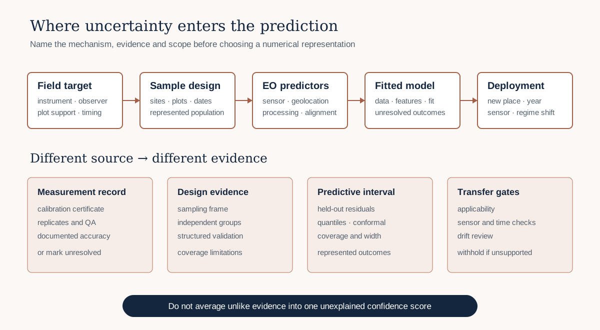
The diagram follows one prediction from ecological observation to deployment. Some sources can be propagated numerically when their measurement models are documented. Others are assessed through repeated sampling, structured validation, interval coverage, applicability or drift evidence. A box labelled “unquantified” is more honest than an invented contribution.

5. Six uncertainty families in predictive EO

Measurement uncertainty

Variation and possible bias in the target or predictor measurement: instrument accuracy, observer differences, laboratory calibration, geolocation error and temporal mismatch. A residual-based interval may contain some effects that happened to be present in calibration data, but it does not separately estimate them or guarantee relevance under a new protocol.

Sampling uncertainty

Uncertainty caused by which sites, plots, dates or habitat conditions entered the study. More pixels derived from the same few plots do not create more independent ecological sampling. Structured validation can expose transfer variability; it cannot make a convenience sample probability-based after the fact.

Model uncertainty

Variation caused by limited training data, model family, feature choices, hyperparameters and fitting randomness. Refitting across valid development samples or folds can reveal sensitivity. One fitted ensemble's tree-to-tree spread is not automatically a calibrated prediction interval.

Residual or outcome uncertainty

Variation in the target not resolved by the available predictors and fixed model. Prediction intervals commonly target this outcome-level variation. It may be heterogeneous: wet, short vegetation can have a different residual distribution from tall, structurally complex vegetation.

Spatial uncertainty

Uncertainty related to spatial support, location error, unresolved spatial processes and transfer to new places. A dense cluster of nearby rows can make row-wise evidence look abundant while providing little independent spatial replication.

Extrapolation and temporal-transfer uncertainty

Uncertainty when predictor combinations, sensors, seasons, management regimes or years differ from calibration. Ordinary interval methods may remain narrow during shift. Chapter 5 applicability and Chapter 7 drift gates therefore remain separate blocking evidence.

6. Worked example — build an uncertainty register

Predict before running

Suppose a residual interval is calibrated from held-out plots acquired with one sensor in 2024. Which register rows may be partly represented by the interval? Which remain separate limitations for a 2027 sensor transfer?

uncertainty_register = [
    {"source": "field measurement", "type": "measurement",
     "represented_by_interval": False},
    {"source": "which meadows were sampled", "type": "sampling",
     "represented_by_interval": False},
    {"source": "unexplained held-out variation", "type": "residual",
     "represented_by_interval": True},
    {"source": "new sensor or year", "type": "transfer",
     "represented_by_interval": False},
]
for item in uncertainty_register:
    print(item["type"], "→", item["represented_by_interval"])

Code walkthrough

1. The register contains one row per identifiable uncertainty source.
2. source names the concrete event or process rather than using “data uncertainty” as a catch-all.
3. type places the source in a shared vocabulary.
4. represented_by_interval asks a narrow evidence question: did the interval design actually include this source under comparable conditions?
5. False does not mean the source is unimportant or absent. It means the proposed interval must not claim to quantify it.
6. The loop prints a reviewable boundary between represented and unrepresented sources.

Extend the operational register with stage, direction, affected output, evidence, numerical representation, diagnostic, mitigation, owner and review trigger.

Diagnostic check

Choose one interval already produced by the project and trace its input labels. If you cannot name which sites, dates, measurement protocols and transfer conditions generated its residual evidence, mark its scope unresolved. Confirm that every source labelled “represented” actually occurred in comparable calibration observations; similarity assumed from subject-matter intuition is not enough.

7. Uncertainty, variability, bias, applicability and ignorance

• Variability describes real differences among ecological units or conditions. It is not always something to eliminate.
• Bias is systematic error under a defined comparison. A narrow interval centred on a biased prediction remains problematic.
• Predictive uncertainty describes outcome dispersion under the fitted procedure and its assumptions.
• Applicability describes whether the prediction unit resembles represented evidence under the Chapter 5 support rule.
• Ignorance marks a limitation that current evidence cannot credibly quantify.

A single “confidence score” that mixes these concepts usually hides how it was produced. Preserve them as separate fields or layers with explicit release rules.

8. What a predictive interval does—and does not—contain

An interval calibrated from protected held-out residuals represents the empirical residual behaviour of the complete fitted procedure for observations exchangeable, or sufficiently comparable, with that calibration design. The exact scope depends on how training, calibration and assessment were sampled and separated.

It does not automatically represent:

• target measurement error absent from the supplied metadata;
• unobserved regions, seasons, sensors or management regimes;
• causal uncertainty about ecological mechanisms;
• geolocation error not present in calibration;
• future changes in the target–predictor relationship;
• the probability that one realised interval contains its fixed unknown target.

Lessons 3.23–3.24 will evaluate interval procedures across repeated protected observations. Lesson 3.25 will combine intervals with applicability without merging their meanings.

Check your understandingCan one residual interval automatically represent measurement, sampling, model and transfer uncertainty?

Choose one answer

No; its scope depends on the data, fitting procedure and evaluation designYes; every interval includes all uncertaintyYes, when it is labelled 90%

Check answer

9. Design an uncertainty inventory

For each source, record:

1. stage: field, EO acquisition, preprocessing, sampling, model, transfer or communication;
2. mechanism: what can vary or be wrong;
3. affected quantity: target, predictor, prediction, bound, support state or decision;
4. evidence: calibration certificate, replicate, metadata, fold result, residual diagnostic, applicability or drift record;
5. representation: distribution, interval, sensitivity analysis, categorical flag or unresolved limitation;
6. scope: sites, dates, sensors and prediction units for which the evidence is relevant;
7. mitigation: improve measurement, redesign sampling, refit, widen/condition an interval, review or withhold;
8. trigger: the condition requiring renewed evidence.

Do not add uncertainty contributions by arithmetic unless their scales, dependence and propagation model justify it. “±2 cm field error + ±5 cm model error = ±7 cm total” is not a general rule.

10. Model clinic — “our model is 90% confident”

The project report states: “The model is 90% confident that vegetation height is 18–26 cm.” Diagnose the statement.

• Problem: the wording does not name the interval method, target population, calibration evidence or coverage interpretation.
• Evidence needed: interval construction, nominal target, empirical coverage and width on protected structured evidence, group failures and applicability status.
• Consequence: readers may interpret a long-run coverage procedure as a probability that this particular interval is correct.
• Fix: write, for example: “The split-conformal procedure targeted 90% marginal coverage and achieved 88% across 50 protected observations from four represented sites; coverage at one site was 70%. This cell is inside the declared applicability domain.”

The revised statement is longer because the claim is more precise.

11. Common mistakes

Calling disagreement among trees a prediction interval

Why beginners make it: ensembles expose many component predictions. Recognition: the interval is the tree percentile with no outcome calibration. Fix: treat component spread as a model diagnostic unless a validated method links it to outcome coverage. Consequence: interval width can be severely miscalibrated.

Treating fold-to-fold metric spread as pixel uncertainty

Why: both involve variation. Recognition: one RMSE standard deviation is attached to every pixel. Fix: report fold spread as procedure-stability evidence and construct prediction-unit intervals separately. Consequence: local heterogeneity disappears.

Inflating intervals to repair extrapolation

Why: a larger number feels conservative. Recognition: unsupported cells receive an arbitrary multiplier. Fix: preserve the applicability gate and seek relevant calibration evidence. Consequence: unsupported predictions gain an unjustified appearance of quantified reliability.

Describing 90% marginal coverage as 90% coverage in every habitat

Why: the nominal level looks universal. Recognition: no subgroup counts or intervals are reported. Fix: examine structured groups with sufficient evidence and state marginal versus conditional scope. Consequence: vulnerable subgroups can be hidden by pooled results.

Inventing target-measurement precision

Why: a complete inventory feels required. Recognition: a numerical field error appears without protocol evidence. Fix: mark it unresolved and request documentation. Consequence: a fabricated number propagates through the model package.

12. Guided practice — audit the Environmental Monitoring Project

1. Add ## Lesson 3.22 checkpoint to the cumulative notebook.
2. Copy the frozen prediction contract, feature schema, validation claim and applicability rule into the checkpoint by reference and version.
3. Trace one target observation from field measurement through join, model fitting and held-out prediction.
4. Identify at least eight uncertainty sources across the evidence chain.
5. Classify each source without forcing it into only one family when mechanisms overlap.
6. Record whether the current residual interval is expected to represent it, partly represent it or not represent it.
7. Provide the evidence supporting that judgement.
8. Mark undocumented measurement accuracy and community-code meaning as unresolved rather than inventing values.
9. Separate systematic bias from dispersion.
10. Identify which sources require a numerical interval, sensitivity analysis, applicability flag, drift gate or written limitation.
11. State the target interval claim for Lesson 3.23.
12. State the calibration population required for that claim.
13. Define at least three structured coverage summaries for Lesson 3.24.
14. Write a release trigger for a new sensor, year and outside-applicability cell.

13. Independent challenge — same model, three destinations

Evaluate the same fitted model for:

• additional plots at represented 2024 sites;
• a new coastal region acquired in 2024;
• represented sites acquired by a replacement sensor in 2027.

For each destination, state which uncertainty sources are plausibly represented by existing held-out residuals, which are threatened by shift, which applicability evidence is needed and whether a numerical interval claim can be released. Do not solve missing evidence by choosing an arbitrary wider interval.

14. Scientific interpretation

An uncertainty inventory is a model of the evidence chain, not proof that every source can be quantified. Its scientific value lies in preventing a residual interval from carrying claims it was not designed to support. This discipline also guides efficient improvement: replicate uncertain measurements, expand underrepresented sampling, improve predictors for structured residuals, collect calibration evidence in the transfer domain or withhold unsupported use.

Check your understandingWhat is the strongest response to predictions from a sensor regime absent from calibration?

Choose one answer

Flag a transfer limitation and require new evidence rather than inflating an arbitrary intervalMultiply every interval by twoCall the map 95% confident

Check answer

15. Submission

Submit:

• the executed Lesson 3.22 notebook checkpoint;
• uncertainty_register.csv with stage, source, type, affected output, evidence, representation, scope, mitigation and trigger;
• UNCERTAINTY_INVENTORY.md explaining at least eight project-specific sources;
• uncertainty_claim_boundary.md stating exactly what the Chapter 6 interval will and will not represent;
• a short comparison of the three transfer destinations.

The submission fails if it treats uncertainty as error, calls an unsupported score confidence, invents measurement precision, merges applicability into interval width or claims that one interval represents every source.

16. Portfolio artifact

Prediction Evidence Package — Uncertainty Inventory

This first component records where uncertainty enters, which evidence can represent it and where the project must use limitations or release gates. Lesson 3.23 will add conditional-quantile interval evidence.

17. Reflection

1. Which uncertainty source is most likely to be hidden by a large row count?
2. When is a wide interval scientifically appropriate?
3. Why can a narrow interval be untrustworthy outside applicability?
4. Which source in your project is currently ignorance rather than quantified uncertainty?
5. What new evidence would convert it into an estimable quantity?

18. Core references

• Gneiting and Raftery (2007), probabilistic forecasts and proper scoring rules
• IPCC guidance note on consistent treatment of uncertainty
• JCGM publications on measurement uncertainty

Further advanced reading

• O'Hagan (2012), probabilistic uncertainty specification
• Meyer and Pebesma (2021), area of applicability

19. Tested software versions and evidence status

The worked register uses core Python and was reviewed for Python 3.12.13. Later chapter examples use NumPy 2.4.2, pandas 2.2.3, scikit-learn 1.9.0 and XGBoost 3.3.0. The training pack is synthetic and CC0-1.0. The published Baltic dataset informs the continuing scientific setting but does not supply documented uncertainty values to this teaching pack.

20. Professional standard

A defensible uncertainty statement identifies the quantity, method, evidence population, nominal target, empirical performance, structured failures, applicability and unrepresented sources. If one of these is unknown, name the limitation instead of replacing it with confident language.