Domain of Applicability and Extrapolation

1. Problem — a model can predict everywhere that a raster has pixels

Learning outcome

By the end of this lesson, you will be able to distinguish geographic interpolation from environmental interpolation; audit univariate predictor ranges; calculate a scaled multivariate nearest-training-analogue distance; define an applicability threshold from development evidence consistent with the validation design; classify prediction units as supported, review or outside applicability; produce a Domain of Applicability map; and prevent visually complete predictions from implying uniform evidential support.

• Lesson type: Domain of Applicability Signature Laboratory
• Estimated time: 250–340 minutes
• Prerequisites: Lessons 3.3, 3.10, 3.15 and 3.17–3.20; Module 2 aligned raster stack and NoData contracts
• Portfolio outputs: applicability_threshold.json, nearest_analogue.csv, domain_of_applicability.tif, applicability_map.png, and DOMAIN_OF_APPLICABILITY.md

Why this matters

Once a fitted model receives a complete raster stack, it will normally return a number for every valid pixel. Software success is not scientific support. A coastal cell may contain a spectral, height and moisture combination never represented in training. A new site can lie near sampled geography but occupy novel environmental space. Conversely, a geographically distant site can resemble represented conditions.

Interpolation and extrapolation therefore need two coordinate systems: geographic space and predictor space. Distance from a field plot alone does not define support, and each predictor falling inside its separate range does not guarantee the multivariate combination was observed.

A professional prediction release places an applicability layer beside the prediction. Unsupported areas are flagged or masked according to a declared policy. This may produce a less complete-looking map, but it is a more complete statement of evidence.

Core lesson: the map of where the model knows enough is as important as the map of what it predicts.

Mental model

training predictor space + validation design
                  ↓
range checks + scaled nearest analogue + threshold
                  ↓
 prediction-grid feature vector for every valid unit
                  ↓
       supported · review · outside applicability
                  ↓
 prediction layer + support layer + explicit use policy

2. Scientific context — moving from sampled meadows to a prediction grid

The Environmental Monitoring Project now has a fixed feature schema and model. The intended map consists of aligned 10 m prediction units. The raster grid, CRS, transform, masks, resampling and NoData behaviour were established in Module 2; this lesson does not reteach them.

For each valid prediction unit, assemble predictors in the saved order and units. Compare them with the outer-development training evidence that would be available at deployment. Do not include the target, post-outcome measurements or final-test data in the support model.

The teaching grid and training table are synthetic. Their novel coastal zone is intentionally obvious enough to practise a conservative gate. The resulting map is not an applicability assessment of real Baltic meadows.

3. Concept — interpolation and extrapolation have several meanings

Geographic interpolation

A prediction lies between or near sampled locations. This can help when environmental processes vary smoothly, but proximity does not guarantee similar habitat, management, sensor conditions or predictor values.

Geographic extrapolation

A prediction lies beyond sampled geography. It may face new spatial processes, but geographic distance alone does not prove predictor novelty.

Univariate environmental interpolation

Every predictor lies within its observed training minimum and maximum. This is a necessary first check for many models, not a sufficient multivariate guarantee.

Multivariate environmental interpolation

The combination of predictor values is similar to at least one represented training analogue after appropriate scaling and feature selection. This is stronger than range checks but depends on the distance metric, scaling, feature redundancy and definition of similarity.

Environmental extrapolation

One or more predictors, or their multivariate combination, lies beyond the support used to estimate performance. Tree ensembles still output values by extending terminal-node predictions. The absence of a software error is not evidence of reliable transfer.

Check your understandingEvery predictor is within its separate training range. Is multivariate support guaranteed?

Choose one answer

No; their combination may still lack a close training analogueYes; univariate ranges prove interpolationYes, if the pixel is geographically near a plot

Check answer

4. Visual explanation — a prediction map needs a companion support map

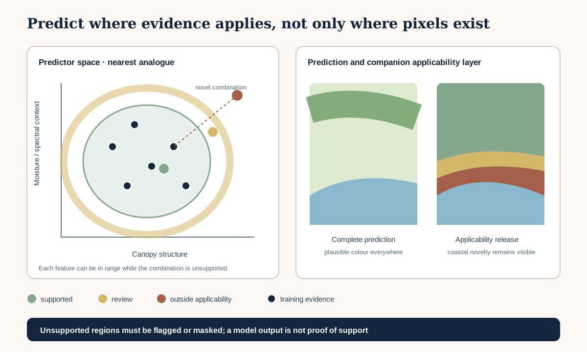
The first panel shows a two-feature simplification. Real applicability is multivariate. The second shows how an unsupported coastal band can still receive plausible green prediction values. The release panel replaces false completeness with a review or mask class and retains a transparent reason code.

5. Worked example — calculate a scaled nearest-analogue distance

Predict before running

One new cell is within the training range for every predictor but combines very high canopy height with very low NDVI, a combination never observed. Will univariate checks flag it? Could multivariate nearest-neighbour distance flag it?

import numpy as np
from sklearn.preprocessing import StandardScaler

features = ["sentinel2_ndvi", "uav_height_p95", "moisture_index"]
scaler = StandardScaler().fit(X_development[features])
training_z = scaler.transform(X_development[features])
prediction_z = scaler.transform(prediction_units[features])

distance = np.sqrt(
    ((prediction_z[:, None, :] - training_z[None, :, :]) ** 2).sum(axis=2)
)
prediction_units["nearest_training_distance"] = distance.min(axis=1)
prediction_units["nearest_training_row"] = distance.argmin(axis=1)
prediction_units[["nearest_training_distance", "nearest_training_row"]].head()

Code walkthrough

1. The feature list is the frozen operational schema subset used for this declared support rule.
2. StandardScaler is fitted only on development training evidence.
3. Scaling prevents centimetre-valued features from dominating unitless indices solely because of numeric magnitude.
4. Training and prediction units receive the same transformation.
5. Broadcasting creates every prediction-to-training difference vector.
6. Squaring and summing produces squared Euclidean distance in standardized predictor space.
7. The square root returns distance.
8. .min(axis=1) finds the closest represented training analogue for every prediction unit.
9. .argmin(axis=1) preserves which training row supplied that analogue.
10. The result is a diagnostic index, not a probability of correctness.
11. For large rasters, compute in chunks rather than materialising the full distance matrix; Chapter 7 will operationalise scale.

Diagnostic check

Verify feature order, units, transformations, missing-value handling and scaler provenance. Correlated features can receive repeated weight in Euclidean distance. Document whether features are grouped, reduced or weighted from development evidence. Confirm the closest analogue belongs to permitted training roles and not the final test.

6. Univariate range checks with reason codes

For each feature, preserve development minimum, maximum and robust quantiles. Flag values below or above the observed range. A robust range such as the 1st–99th percentile can identify sparse tails, but it must not be labelled the literal training range. Use distinct reason codes:

• below_training_min;
• above_training_max;
• sparse_training_tail;
• missing_required_predictor;
• invalid_upstream_qa;
• novel_multivariate_combination.

Do not silently clip prediction values to training bounds. Clipping changes the input while concealing extrapolation. If a transformation mathematically clips values, document it as part of the trained procedure and retain a pre-clipping novelty flag.

7. Define the threshold from development evidence

An applicability threshold must not be chosen from final-test errors. One defensible pattern is to reproduce the validation structure within development data:

1. for each development fold, calculate each held-out row’s distance to that fold’s training rows;
2. collect those cross-validated nearest-analogue distances;
3. relate distance to held-out error or use a predeclared conservative quantile;
4. freeze supported and review thresholds;
5. assess the rule with protected outer predictions;
6. leave the final test sealed until the complete procedure is fixed.

Meyer and Pebesma’s Area of Applicability framework links dissimilarity to the cross-validation design used for performance estimation. The principle is important: the region to which an error estimate applies depends on how training-like held-out observations were defined. Do not copy a universal distance threshold from another dataset.

Create three operational states rather than pretending one boundary is exact:

• supported: distance and all QA/range gates within the frozen support rule;
• review: near the support boundary or affected by a warning that requires expert inspection;
• outside applicability: exceeds a blocking threshold, lacks required predictors or fails upstream QA.

Check your understandingWhere should applicability thresholds be derived?

Choose one answer

From structured development evidence consistent with the validation designFrom repeated inspection of final-test errorsFrom a universal Euclidean-distance value

Check answer

8. Nearest analogue is useful but not complete

A nearby analogue in scaled space does not guarantee prediction quality. The training row may be noisy, a predictor may omit an important process, or the target relationship may differ through time. Applicability is a support diagnostic, not certainty.

Improve the audit by preserving:

• nearest analogue ID and site;
• distance and threshold version;
• feature-specific range flags;
• acquisition and sensor compatibility;
• geographic distance as a separate diagnostic;
• prediction and expected error evidence within distance bands;
• fold-level support behaviour;
• model and feature-schema versions.

Do not let one densely sampled site provide every nearest analogue. Report analogue-site diversity and consider group-aware thresholds when deployment claims transfer to new sites.

9. Build the Domain of Applicability map

Write an aligned categorical raster whose values mean:

• 1 = supported;
• 2 = review;
• 3 = outside applicability;
• 255 = NoData or outside the prediction mask.

Keep the continuous distance layer as a separate analytical output. Publish a legend, CRS, transform, resolution, extent, NoData, feature schema, scaling record, threshold and reason-code table. The applicability grid must align exactly with the prediction grid.

For the public prediction layer, choose and document one policy:

• mask outside-applicability predictions;
• retain values with a prominent flag layer and block decision use;
• show a hatched overlay in a visualisation while delivering machine-readable categories.

Never colour unsupported predictions like supported ones without a conspicuous companion layer. Accessibility requires textual summaries of supported, review and outside proportions and named affected regions.

10. Connect applicability with observed error

Stratify protected outer residuals by the frozen support classes or distance bands. Ask whether error magnitude increases with distance and whether specific sites sit outside support. This is a diagnostic assessment of the rule, not permission to tune it repeatedly on outer evidence.

If error does not increase monotonically, the distance may still detect novelty but may not predict error well. Possible reasons include irrelevant features, inadequate scaling, missing predictors, small evidence or heterogeneous noise. Report that result honestly. A convenient applicability index is not guaranteed to be a universal error model.

Chapter 6 will add uncertainty. Applicability and uncertainty are different: a supported point can have a wide interval, and an extrapolated point can receive a narrow but misleading model-based interval. Both layers belong in the final evidence package.

11. Model clinic — complete maps with incomplete evidence

“Every cell is within each feature’s range”

The feature combination is novel. Add multivariate distance and analogue evidence.

“The closest training point is only 500 m away”

Its habitat and predictor vector are dissimilar. Separate geographic from environmental distance.

“Distance above 3 is always extrapolation”

The threshold was copied without regard to scaling, dimensions or validation design. Derive and version it from current development evidence.

“Unsupported pixels were clipped to look realistic”

Clipping concealed novelty. Restore the original inputs, reason flags and mask policy.

“SHAP explains why the extrapolated prediction is high”

The explainer describes the model output, not its reliability. Applicability warning takes precedence.

“The blank coastal area makes the map look unfinished”

The blank is an evidence result. Improve legend and narrative, not false coverage.

12. Common mistakes

Fitting the scaler on the prediction raster

Why beginners make it: all values are available. Recognition: support thresholds change with the deployment scene. Fix: fit and version scaling from development training data only. Consequence: the definition of novelty moves with the data being judged.

Counting correlated features repeatedly

Why: each column enters distance equally. Recognition: a family of similar indices dominates. Fix: justify reduction, grouping or weights inside development evidence. Consequence: distance measures redundancy more than novelty.

Using final-test errors to choose the threshold

Why: error provides an appealing cutoff. Recognition: multiple thresholds are tried on final labels. Fix: select inside structured development and assess once. Consequence: final performance and coverage are optimistic.

Treating NoData as outside applicability

Why: both are not used. Recognition: sensor absence and environmental novelty share one code. Fix: preserve NoData separately. Consequence: processing failure is confused with model support.

Dropping reason codes

Why: one category map seems enough. Recognition: reviewers cannot tell range failure from missing input. Fix: publish primary reason and all flags. Consequence: remediation is impossible.

13. Guided practice — produce the applicability evidence package

1. Add ## Lesson 3.21 checkpoint to the cumulative notebook.
2. Load the fixed feature schema, development table and synthetic prediction grid.
3. Validate units, transformations, feature order and missing-value rules.
4. Save training minimum, maximum and declared sparse-tail limits per feature.
5. Apply univariate checks and preserve reason codes.
6. Fit scaling only on the permitted development training evidence.
7. Calculate cross-validated nearest-analogue distances using the Chapter 3 groups.
8. Freeze supported, review and outside thresholds with rationale.
9. Calculate each prediction unit’s distance and nearest analogue.
10. Record analogue site and geographic distance separately.
11. Assign applicability state without opening the final test.
12. Write aligned continuous-distance and categorical applicability rasters.
13. Produce a map with prediction, applicability and an explicit unsupported mask.
14. Summarise area/proportion by state and reason.
15. Compare protected outer error across the already frozen states.
16. Write the use policy and limitations.
17. Complete the Chapter 5 handover.

14. Independent challenge — a geographically near but environmentally novel strip

The synthetic coastal strip lies close to training plots yet combines low NDVI, high moisture index and high UAV height. Demonstrate why geographic distance and separate range checks can miss the problem. Identify the nearest environmental analogue, quantify its distance and decide whether to support, review or mask the strip.

Write a short field-sampling proposal that would expand support efficiently. New labels do not retroactively validate the existing map; specify how they would enter a new versioned training and assessment design.

15. Scientific interpretation

The Domain of Applicability map describes similarity to represented training evidence under a declared feature space, scaling rule, threshold and validation design. It does not guarantee correctness inside the supported area or prove incorrectness outside it. It tells reviewers where the reported performance has a plausible support relationship and where the model is extrapolating.

The release is scientifically stronger when unsupported regions remain visible as unsupported. A complete-looking prediction raster without this layer implies equal reliability the evidence cannot provide. Chapter 6 will quantify several forms of uncertainty while keeping applicability as a separate concept.

16. Submission

Submit:

• the executed Lesson 3.21 notebook checkpoint;
• applicability_threshold.json with schema, scaler, fold design, quantiles, thresholds and versions;
• nearest_analogue.csv with unit ID, distance, analogue ID/site and reason codes;
• domain_of_applicability.tif plus metadata and aligned NoData contract;
• applicability_map.png with accessible description and textual coverage summary;
• DOMAIN_OF_APPLICABILITY.md defining states, evidence, use policy, limitations and sampling recommendation;
• the complete Chapter 5 Model Diagnostic and Applicability Package.

The submission fails if it fits scaling on deployment data, hides unsupported units, mixes NoData with extrapolation, uses final-test labels to tune thresholds or presents the support index as a probability of accuracy.

17. Portfolio artifact

Model Diagnostic and Applicability Package — Complete Chapter 5 Package

The package combines regression evidence, class and probability quality, structured failure, interpretation boundaries and the Domain of Applicability map. It answers: how does the fixed procedure perform, where does it fail, what does it rely on, and where is its evidence relevant? Chapter 6 will add prediction uncertainty without collapsing it into applicability.

18. Reflection

1. How can a geographically close unit be environmentally novel?
2. Why are separate feature ranges insufficient for multivariate support?
3. Which data are permitted to fit scaling and select thresholds?
4. What is the difference between NoData and outside applicability?
5. Which region should receive new sampling first, and why?

Check your understandingHow should outside-applicability predictions be released?

Choose one answer

Flagged or masked with reason codes and a machine-readable support layerColoured exactly like supported predictionsReplaced silently by the nearest training value

Check answer

19. Core references

• Meyer and Pebesma (2021), estimating the area of applicability
• scikit-learn 1.9 — StandardScaler
• scikit-learn 1.9 — nearest neighbours

Further advanced reading

• Meyer et al. (2018), improving performance of spatio-temporal ML models
• Roberts et al. (2017), structured cross-validation
• CAST documentation — area of applicability

20. Tested software versions

Teaching examples were reviewed for Python 3.12.13, JupyterLab 4 / Notebook 7, NumPy 2.4.2, pandas 2.2.3 and scikit-learn 1.9.0. Raster delivery uses the existing Module 2 tested geospatial stack. All predictor vectors, coordinates, distances and labels are deterministic synthetic teaching evidence, not a real Baltic applicability analysis.