Prediction Intervals and Quantile Approaches

1. Problem — one expected value cannot describe predictive spread

Learning outcome

By the end of this lesson, you will be able to distinguish a point prediction, conditional quantile, prediction interval and confidence interval; explain pinball loss; fit lower and upper XGBoost quantile models with a frozen feature and validation contract; detect quantile crossing; calculate empirical coverage and interval width on protected structured evidence; and judge calibration and sharpness together.

• Lesson type: Quantile Prediction Interval Laboratory
• Estimated time: 240–330 minutes
• Prerequisites: Lessons 3.8, 3.12–3.15, 3.17, 3.21 and 3.22
• Portfolio outputs: quantile_predictions.csv, QUANTILE_INTERVAL_REPORT.md, quantile_coverage_by_group.csv and the Lesson 3.23 notebook checkpoint

Why this matters

Two meadow cells can receive the same point prediction but have very different plausible outcome ranges. One may lie among dense, consistent training analogues; the other may occupy conditions where held-out vegetation measurements varied widely. A decision about field review, grazing management or monitoring priority needs more than the centre of the predictive distribution.

Quantile regression estimates selected parts of that conditional distribution directly. It can allow intervals to widen and narrow with predictors, unlike one constant residual band. But an interval is useful only if protected observations achieve adequate coverage without becoming so wide that the result loses decision value.

Core lesson: evaluate interval calibration and sharpness together, under the same transfer structure as the prediction claim.

Mental model

frozen predictors + lower quantile objective → lower bound
frozen predictors + upper quantile objective → upper bound
                                  ↓
       protected outcomes → coverage · width · miss direction
                                  ↓
              calibrated enough and useful enough?

The two fitted bounds are candidate interval components. Only protected outcome evidence establishes whether the complete procedure deserves an interval claim.

2. Scientific context — conditional spread in meadow structure

The Environmental Monitoring Project retains its fixed target, feature order, spatial groups and sealed final test. The synthetic training data include heterogeneous residual variation: structurally complex meadow conditions are deliberately harder to predict than homogeneous short vegetation. This allows the lesson to test whether interval width responds to predictors.

The target unit remains whatever the project's target specification documents. If the real published metadata does not establish a unit for a selected variable, use the explicit neutral label “target units”; do not convert tutorial values into an undocumented centimetre or biomass unit.

3. Concept — four different statistical objects

Point prediction

A single estimate such as a conditional mean or median. Its meaning depends on the training objective.

Conditional quantile

For predictors $X=x$, the $\tau$-quantile $q_\tau(x)$ is a value intended to satisfy:

$$P(Y \le q_\tau(x) \mid X=x) = \tau$$

under the represented data-generating conditions. A 0.90 quantile is not a 90% probability that the model is correct.

Prediction interval

The pair $[q_{0.10}(x), q_{0.90}(x)]$ targets a central 80% outcome interval. It concerns a new outcome, including residual variation represented by training and evaluation.

Confidence interval

A confidence interval usually concerns an estimated parameter, such as a mean or coefficient. It is not a synonym for a prediction interval. Prediction intervals are generally wider because individual outcomes vary around the conditional centre.

Check your understandingWhat does a fitted 0.90 conditional quantile estimate?

Choose one answer

A value below which about 90% of outcomes are intended to fall for represented predictor conditionsA 90% probability that the model is correctThe upper 90% confidence bound for the mean

Check answer

4. Visual explanation — intervals must be checked in two directions

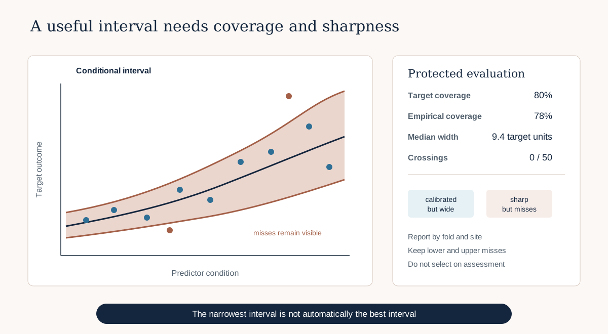
The first panel asks whether bounds adapt to predictor conditions. The second asks how frequently protected outcomes fall inside. A narrow band with many misses is sharp but miscalibrated. A very wide band with complete coverage may be calibrated conservatively but uninformative. The aim is the narrowest useful interval consistent with the declared coverage evidence—not narrowness alone.

5. Pinball loss — asymmetric penalties estimate a quantile

For residual $u = y - q_\tau(x)$, quantile or pinball loss is:

$$L_\tau(u) = \begin{cases} \tau u, & u \ge 0 \\ (\tau - 1)u, & u < 0 \end{cases}$$

At $\tau=0.90$, underpredicting a value is penalised more strongly than overpredicting by the same amount. The fitted function therefore moves upward toward the conditional 90th percentile. At $\tau=0.50$, the loss is proportional to absolute error and targets a conditional median.

Quantile regression does not require normally distributed residuals or constant variance. It still requires relevant training evidence, appropriate model complexity and honest evaluation.

6. Worked example — fit lower and upper XGBoost quantiles

Predict before running

If uncertainty increases in tall, heterogeneous vegetation, should the 0.10 and 0.90 fitted quantiles stay a constant distance apart? What evidence would show whether they adapt usefully?

from xgboost import XGBRegressor

def fit_quantile(alpha):
    model = XGBRegressor(
        objective="reg:quantileerror", quantile_alpha=alpha,
        tree_method="hist", n_estimators=400, learning_rate=0.04,
        max_depth=3, random_state=42, n_jobs=1,
    )
    return model.fit(X_train[feature_order], y_train)

lower_model = fit_quantile(0.10)
upper_model = fit_quantile(0.90)
lower = lower_model.predict(X_assessment[feature_order])
upper = upper_model.predict(X_assessment[feature_order])

Code walkthrough

1. XGBRegressor uses the same ordered operational features as the point model.
2. The function makes the quantile level explicit and reproducible.
3. XGBoost 3.3 uses reg:quantileerror with quantile_alpha for quantile loss.
4. The histogram tree method follows the official quantile example; avoid assuming every tree method behaves equally for this objective.
5. Complexity settings belong to a development-only protocol, not repeated inspection of assessment coverage.
6. The fixed random seed and one worker support reproducibility.
7. Lower and upper models are fitted only on the permitted training role.
8. The assessment feature schema is validated before prediction.
9. The outputs are bounds, not yet verified intervals. Coverage evidence gives them scientific meaning.

You may also fit several quantiles through supported current XGBoost APIs, but a single call does not remove the need to document output order, detect crossing and evaluate each interval.

Diagnostic check

Before calculating coverage, assert that observation IDs and bound predictions join one-to-one and that no outer assessment label entered preprocessing, early stopping, hyperparameter choice or crossing repair. Plot lower and upper predictions against the point prediction. Unexpected discontinuities, identical bounds or widths unrelated to known residual structure are investigation prompts—not reasons to delete rows.

Repeat the check by outer fold. A quantile model that behaves sensibly in pooled data can collapse at the only truly new site. Preserve raw bound predictions so the failure remains reproducible after summaries are produced.

7. Calculate coverage, width and misses

For observation $i$:

$$c_i = I(l_i \le y_i \le u_i), \qquad w_i = u_i-l_i$$

Empirical coverage and mean width are:

$$\widehat{C} = \frac{1}{n}\sum_i c_i, \qquad \overline{W} = \frac{1}{n}\sum_i w_i$$

Report at least:

• nominal coverage target and alpha levels;
• observation and independent-group counts;
• pooled empirical coverage;
• mean and median width;
• width quantiles and maximum;
• lower-side and upper-side miss counts;
• quantile-crossing count;
• coverage and width by held-out site, fold, habitat and applicability state when estimable.

Small subgroup estimates are descriptive and uncertain. Preserve counts rather than presenting a two-row subgroup's 100% coverage as a reliable guarantee.

8. Calibration and sharpness

Calibration asks whether observed outcomes fall within intervals at about the declared rate over the relevant population. Sharpness asks how concentrated the predictive distributions or intervals are, subject to calibration.

An 80% interval covering 40% is too narrow or badly transferred. An 80% interval covering 100% with an enormous width may be conservative but scientifically weak. Neither coverage nor width alone ranks procedures responsibly.

Compare interval methods using protected evidence and a predeclared score. Proper scoring rules such as the interval score can combine width with penalties for misses, but still report the interpretable components. Do not optimise a new method repeatedly against the final test.

Check your understandingWhich interval result is automatically better?

Choose one answer

Neither narrow nor wide alone; coverage, width, subgroup behaviour and decision use must be judged togetherThe narrowest intervalThe interval with 100% coverage regardless of width

Check answer

9. Quantile crossing

Separately fitted lower and upper models can produce $l_i > u_i$. Crossing is not a harmless display problem. It shows that the fitted quantile functions are internally inconsistent at that prediction unit.

Record where crossing occurs and examine feature support, sample size and model complexity. Possible development-stage responses include joint multi-quantile methods, monotonic rearrangement or a documented post-processing rule evaluated on fresh protected evidence. Silently sorting the two predictions hides the failure and changes the model procedure after inspection.

Check your understandingA lower-quantile prediction exceeds the upper-quantile prediction. What should happen?

Choose one answer

Record quantile crossing as a model failure and investigate itSilently swap the two valuesDrop the assessment row

Check answer

10. Validation design remains part of the interval model

Quantile models require the same spatial, grouped and temporal discipline as point models. Random rows from the same field plot can make coverage appear excellent because training and assessment share local conditions. Use the frozen outer folds from Chapter 3 and keep quantile hyperparameter selection inside the inner development loop.

For every outer fold:

1. fit preprocessing and the two quantile models on outer development rows;
2. make bound predictions for untouched outer assessment groups;
3. store observation ID, group, lower, upper and point prediction;
4. concatenate predictions only after every row was predicted out of its training context;
5. evaluate fold and pooled evidence without deleting hard groups.

The sealed final test remains closed until model family, quantiles, tuning, crossing policy and reporting plan are fixed.

11. Intervals and physical constraints

Some environmental targets cannot be negative. Do not clip a negative lower bound silently. Decide inside development whether the model should use an appropriate transformation, constrained objective or a documented post-processing rule. Then evaluate the complete procedure, including coverage near the boundary.

Clipping can increase apparent coverage or create a pile-up at zero. Report pre- and post-rule behaviour and ensure the rule matches the target definition rather than visual preference.

12. Model clinic — the narrowest interval wins

A colleague selects the model with the narrowest mean interval on the outer assessment folds.

• Problem: width is optimised without requiring adequate coverage, and outer assessment has influenced selection.
• Evidence: the narrow model covers only 61% against an 80% target and fails at a wet meadow site.
• Consequence: the interval looks precise while excluding many outcomes and contaminating performance estimation.
• Fix: predeclare a coverage-aware inner-development selection rule, freeze it, and assess the complete procedure on untouched outer evidence.

13. Common mistakes

Calling quantile bounds confidence intervals

Why beginners make it: the phrase is familiar. Recognition: the text says “confidence in the mean” while predicting individual outcomes. Fix: use “prediction interval” and state the conditional quantiles. Consequence: readers misunderstand the statistical object.

Tuning alpha until outer coverage looks good

Why: the nominal level seems adjustable. Recognition: 0.05, 0.10 and 0.15 are tried on the same protected labels. Fix: choose the target from decision needs before assessment. Consequence: reported coverage is optimistic.

Ignoring unequal tail failures

Why: pooled coverage looks sufficient. Recognition: almost every miss is above the upper bound. Fix: report lower and upper misses separately. Consequence: directional bias remains hidden.

Dropping crossing rows

Why: they break interval plots. Recognition: assessment count changes after prediction. Fix: retain and report them as failures. Consequence: the hardest predictions disappear.

Assuming width measures every uncertainty source

Why: width is spatially variable. Recognition: transfer and measurement limitations vanish from the report. Fix: link back to the Lesson 3.22 inventory and Chapter 5 applicability. Consequence: a model property is mistaken for complete knowledge.

14. Guided practice — build the quantile interval report

1. Add ## Lesson 3.23 checkpoint to the cumulative notebook.
2. Load the frozen feature schema and structured outer-fold registry.
3. State the lower and upper quantiles and resulting nominal central coverage.
4. Verify that target and prediction units retain documented meaning.
5. Fit preprocessing and quantile models only inside each outer development role.
6. Preserve hyperparameter selection inside inner groups.
7. Predict lower and upper bounds on untouched outer assessment rows.
8. Save observation ID, fold, site, point prediction, lower and upper.
9. Count crossing before applying any rule.
10. Calculate pooled and fold coverage.
11. Calculate mean, median and 90th-percentile width.
12. Count lower-side and upper-side misses.
13. Summarise coverage and width by site and applicability state with counts.
14. Plot observed values with intervals ordered by site, not by a visually convenient deletion.
15. Compare interval width with absolute residual without claiming width causes error.
16. Write the represented and unrepresented uncertainty sources.
17. Keep the final test sealed.

15. Independent challenge — two intervals with the same coverage

Two candidate procedures both achieve 80% pooled outer coverage. Method A has a smaller median width but fails badly at one independent site. Method B is wider overall but more stable across sites. Use fold counts, interval-score components, applicability and the intended destination to recommend one, recommend neither or restrict their use. Do not collapse the decision into one pooled number.

16. Scientific interpretation

Conditional quantile intervals describe outcome variation learned from represented predictor and target relationships. Their width can adapt to heteroscedastic conditions, but this does not guarantee calibration at a new site, season or sensor. Protected structured coverage is the evidence; the objective name is not.

Narrower intervals are valuable only when their coverage and transfer behaviour remain adequate for the intended decision. Quantile intervals also remain separate from applicability: a narrow interval outside the training domain can be strongly misleading.

17. Submission

Submit:

• the executed Lesson 3.23 notebook checkpoint;
• quantile_predictions.csv with observation, fold, group, point, lower, upper, width, covered and crossing fields;
• quantile_coverage_by_group.csv with counts, coverage, width and miss direction;
• QUANTILE_INTERVAL_REPORT.md documenting objectives, alphas, feature schema, tuning roles, coverage, sharpness, crossing and limitations;
• one accessible interval figure and text alternative.

The submission fails if it tunes on protected assessment, drops crossing or missed rows, reports only width, calls bounds confidence intervals for a mean or implies coverage outside the represented domain.

Reflection

1. Which scientific decision determines the useful nominal interval level?
2. Why can two models with equal coverage have different professional value?
3. What does a concentration of upper-side misses suggest?
4. How would a physical lower boundary change the procedure and its evaluation?
5. Which transfer group most challenges the interval claim?

18. Portfolio artifact

Prediction Evidence Package — Quantile Interval Report

The report adds adaptive lower and upper predictive bounds to the uncertainty inventory. Lesson 3.24 will calibrate intervals using held-out nonconformity scores and examine the assumptions behind empirical coverage.

19. Core references

• XGBoost 3.3, quantile regression example
• XGBoost 3.3, quantile objective parameters
• Koenker and Bassett (1978), regression quantiles

Further advanced reading

• Gneiting and Raftery (2007), proper scoring rules
• scikit-learn, prediction intervals for gradient boosting regression

20. Tested software versions and professional standard

The code pattern was reviewed against XGBoost 3.3.0, which documents reg:quantileerror, quantile_alpha and histogram-tree quantile examples. The chapter environment uses Python 3.12.13, NumPy 2.4.2, pandas 2.2.3 and scikit-learn 1.9.0. Re-run versioned tests before teaching or deploying a different release. A professional interval report makes its nominal target, empirical coverage, width, transfer units, crossing, support and limitations reproducible.