Uncertainty and Applicability Maps

1. Problem — one prediction raster cannot carry the whole evidence claim

Learning outcome

By the end of this lesson, you will be able to explain the different question answered by prediction, lower-bound, upper-bound, interval-width and applicability maps; validate their shared grid and semantic contracts; combine input validity, applicability and uncertainty into transparent release states; prevent narrow extrapolated intervals from implying reliability; evaluate map-level coverage only where reference observations exist; and assemble an accessible, machine-readable Prediction Evidence Package.

• Lesson type: Prediction Evidence Mapping Signature Laboratory
• Estimated time: 250–350 minutes
• Prerequisites: Lessons 3.21–3.24; Module 2 raster alignment, NoData, COG and cartographic QA
• Portfolio outputs: aligned prediction-evidence rasters, prediction_evidence_inventory.csv, PREDICTION_EVIDENCE_PACKAGE.md, accessible map suite and the Chapter 6 notebook handover

Why this matters

A polished prediction map encourages viewers to treat every coloured cell as equally supported. Chapter 5 showed why that is false. Chapter 6 adds another distinction: a prediction interval can be wide inside the training domain and deceptively narrow outside it. Applicability measures similarity to represented evidence; interval width measures dispersion produced by a specified model and calibration procedure. Neither replaces the other.

Professional Earth Observation delivery therefore separates the value being predicted from the evidence qualifying its use. The package must work for a scientist reading a report, an analyst loading rasters, and an automated system enforcing a release gate.

Core lesson: publish the prediction, uncertainty and applicability together, but never collapse them into one unexplained confidence surface.

Mental model

valid predictors → prediction + interval bounds
training similarity → applicability state
prediction + interval + applicability + policy
                     ↓
        supported · review · withhold · NoData

The release state is a governed decision derived from preserved evidence. It is not another probability layer.

2. Scientific context — a decision-ready coastal-meadow map suite

The Environmental Monitoring Project has a fixed point model, quantile or conformal interval procedure, feature schema and Chapter 5 applicability rule. Chapter 2 of Module 2 already taught grid geometry, Rasterio, NoData, alignment and COG validation. This lesson assumes those skills and focuses on modelling semantics.

The synthetic 4 × 6 teaching grid contains supported, review, outside-applicability and NoData units. Values do not represent real Baltic meadow measurements or locations. The grid exists to test whether release logic preserves distinctions under realistic map conditions.

3. Concept — five aligned questions

Prediction map

What value does the fixed model predict for each valid unit? Preserve target name, unit status, prediction unit, model version and timestamp.

Lower- and upper-bound maps

What bounds did the fixed interval procedure produce? A bound is meaningful only with method, nominal target and calibration version.

Interval-width map

How wide is that model-based predictive interval? Width $u-l$ is useful for review prioritisation. It is not a probability of error or support.

Applicability map

How similar is each unit to the represented training evidence under the frozen support rule? It does not quantify residual spread.

Release-state map

What use does the governance policy permit after considering input validity, applicability and uncertainty? This is a transparent decision layer with reason codes, not a new statistical quantity.

Check your understandingWhat does the interval-width map answer?

Choose one answer

How wide the model's represented predictive interval is at each valid prediction unitWhether the unit lies inside training supportWhether ecological change has occurred

Check answer

4. Visual explanation — three evidence layers, one governed release

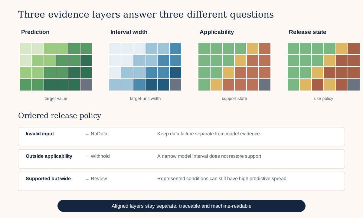
The grid cells occupy identical positions, but the colours answer different questions. The final panel does not average their values. It applies an ordered policy and retains the primary reason for every review or withholding decision.

5. Grid contract — identical geometry is necessary, not sufficient

Every numerical layer must share:

• CRS and axis order;
• affine transform and pixel origin;
• width, height and resolution;
• extent and prediction mask;
• stable cell or unit identifier;
• NoData encoding and validity semantics.

Semantic alignment is equally important:

• same target definition and unit status;
• same prediction unit and temporal support;
• same feature-schema and preprocessing version;
• same model and interval-procedure version;
• same calibration population and nominal coverage target;
• same applicability threshold version;
• clear distinction between source NoData and governance withholding.

Hash the metadata inventory and fail the release if any required contract differs. A correctly aligned raster from the wrong model version is still wrong.

6. Worked example — assign transparent release states

Predict before running

One outside-applicability cell has a narrow interval. Another supported cell has an unusually wide interval. Which should be released, reviewed or withheld?

evidence = prediction_grid.copy()
evidence["interval_width"] = evidence["upper"] - evidence["lower"]
evidence["release_state"] = "supported"
evidence.loc[evidence["interval_width"] > frozen_width_limit,
             "release_state"] = "review"
evidence.loc[
    evidence["applicability_state"] == "outside", "release_state"
] = "withhold"
evidence.loc[evidence["input_valid"] == False,
             "release_state"] = "nodata"

assert evidence[["prediction", "lower", "upper"]].notna().all(axis=1).equals(
    evidence["input_valid"]
)

Code walkthrough

1. The table contains one row per fixed grid unit.
2. Width is derived from the saved bounds rather than entered independently.
3. Valid, supported and adequately narrow units begin in the supported state.
4. The width threshold was frozen using development evidence and decision needs.
5. Wide intervals request review; they do not automatically prove error.
6. Outside applicability overrides narrowness and withholds decision use.
7. Invalid input overrides every model state and remains NoData.
8. The assertion verifies that numerical predictions exist exactly for input-valid rows.

Production code should also assign one primary reason and retain all secondary reason flags. The policy order must be versioned and tested.

Diagnostic check

Choose five grid units representing supported/narrow, supported/wide, review, outside/narrow and NoData states. Trace every displayed cell back to model, interval, applicability and input records. Confirm that changing the map colour scale cannot change release state and that a public mask does not erase the underlying analytical value or reason code from the audit package.

7. Why narrow intervals cannot rescue extrapolation

Quantile and split-conformal intervals learn from represented training and calibration relationships. A novel predictor combination can fall into tree leaves that produce stable-looking bounds even though transfer evidence is absent. A constant-width symmetric conformal interval will be identical inside and outside applicability by construction.

Therefore:

• supported + narrow: may be released under the documented purpose;
• supported + wide: valid support but high represented predictive dispersion; review or restrict the decision;
• outside + narrow: potentially overconfident extrapolation; withhold or flag prominently;
• outside + wide: both extrapolation and high model-based dispersion; withhold;
• NoData: no valid model input; do not call it uncertainty or extrapolation.

Check your understandingA cell is outside applicability but has a narrow interval. What is the defensible release state?

Choose one answer

Withhold or prominently flag it because model-based narrowness does not restore supportRelease it as high confidenceReplace the interval with NoData and call the inputs missing

Check answer

8. Set an uncertainty review rule without test peeking

A width threshold is a governance decision, not a universal statistical constant. Derive it from:

• the target unit and decision tolerance;
• development interval-width distribution;
• error and coverage behaviour across width bands;
• operational cost of unnecessary review versus unrecognised risk;
• minimum independent evidence in each relevant group.

Freeze the rule before final assessment. A 90th development percentile can be a transparent review trigger, but it does not mean the widest 10% are wrong. If a decision has a maximum tolerable range in target units, document why that range matters scientifically.

Do not choose the threshold to make the published map look complete.

9. Validate the numerical relationships

For every input-valid unit, assert:

• lower ≤ upper;
• width = upper − lower within numeric tolerance;
• point prediction lies between bounds when the chosen method is expected to include it;
• all values are finite and use the declared dtype;
• categorical states use the documented code table;
• outside-applicability and review areas retain their reasons;
• invalid input never receives a released prediction.

For physical target constraints, apply only the frozen evaluated rule from Lesson 3.23. Never clip a map silently after evaluation.

10. Map empirical evidence without inventing pixel truth

Coverage can be evaluated only where independent reference outcomes exist at compatible spatial and temporal support. Do not compare a plot target with every intersecting pixel as though each were an independent validation event.

Create an observation-level assessment table linked one-to-one to the corresponding prediction unit or documented support aggregation. Map covered and missed observations, but avoid interpolating the binary coverage result into unsampled space. Summarise:

• number of reference observations and independent sites;
• nominal and empirical coverage;
• lower- and upper-side misses;
• coverage and width by site, fold and applicability;
• geographic clusters of misses as diagnostic—not causal—evidence.

The raster shows predicted uncertainty; reference points show where empirical coverage was tested.

11. Cartographic and accessibility standard

Use separate, readable panels rather than a rainbow composite:

• a perceptually ordered sequential palette for continuous prediction;
• a different ordered palette for interval width;
• discrete, colour-blind-conscious categories for supported, review, outside and NoData;
• a governed release map using patterns or borders as well as colour where possible.

Every public figure needs:

• descriptive title and subtitle naming target and time;
• units or explicit undocumented-unit wording;
• legend with numerical bounds and category meanings;
• scale, orientation and location context appropriate to the product;
• model, interval and applicability version;
• textual summary of coverage and area/proportion by release state;
• concise alternative text that communicates the important spatial pattern.

Do not use opacity alone to encode support. Low vision, print reproduction and overlapping basemaps can erase the distinction.

12. Package design

The Prediction Evidence Package should contain:

• prediction.tif;
• prediction_lower.tif and prediction_upper.tif;
• prediction_interval_width.tif;
• domain_of_applicability.tif;
• release_state.tif;
• release_reason.tif or a linked reason table;
• prediction_evidence_inventory.csv;
• coverage_assessment.csv;
• accessible PNG/SVG overview and text alternative;
• PREDICTION_EVIDENCE_PACKAGE.md;
• machine-readable metadata, checksums and environment/model identifiers.

Deliver analytical values even when the public visualisation masks withheld cells. Governance masking must not erase the audit trail.

Check your understandingWhich package is decision-ready?

Choose one answer

Aligned prediction, lower, upper, width, applicability, valid-mask and release-state layers with metadata and text summaryA prediction PNG without machine-readable evidenceOne confidence heatmap combining every limitation

Check answer

13. Model clinic — one confidence map

A designer combines normalised interval width and applicability distance into one 0–100 “confidence” score.

• Problem: unlike quantities with different assumptions have been averaged.
• Evidence lost: actual target-unit width, calibration coverage, support reason, NoData and policy threshold.
• Consequence: a moderate score cannot reveal whether a cell is extrapolated, merely wide or missing input.
• Fix: retain separate evidence layers and a categorical release decision with reasons. A dashboard can place them side by side without mathematical fusion.

14. Common mistakes

Mapping standard deviation of trees as calibrated uncertainty

Why beginners make it: the values form a convenient raster. Recognition: no outcome coverage assessment exists. Fix: label it model-spread diagnostic or calibrate a defensible interval method. Consequence: colour implies evidence the method does not have.

Giving withheld cells the same prediction colour

Why: the analytical value still exists. Recognition: the support overlay is optional or hidden. Fix: apply the declared public-release mask while retaining machine-readable analytical layers. Consequence: visually complete output overstates relevance.

Mixing NoData and outside applicability

Why: neither is released. Recognition: both share code 255. Fix: preserve input validity and support state separately. Consequence: data failure and environmental novelty cannot be diagnosed.

Rescaling width per map

Why: each map looks balanced. Recognition: the same colour means different target-unit widths across dates. Fix: use fixed meaningful breaks for comparable products. Consequence: temporal comparison becomes misleading.

Claiming pixel-level coverage without pixel-level targets

Why: maps encourage cell-wise language. Recognition: millions of cells are quoted as validation cases from a few plots. Fix: report the observation support and independent sample count. Consequence: validation precision is invented.

15. Guided practice — assemble the Chapter 6 package

1. Add ## Lesson 3.25 checkpoint to the cumulative notebook.
2. Load the frozen point, interval and applicability procedure metadata.
3. Validate feature schema and input-valid mask.
4. Calculate lower, upper and width for every valid grid unit.
5. join applicability one-to-one by stable unit ID.
6. Assert identical CRS, transform, shape, extent, resolution and NoData contracts.
7. Assert lower/upper/width relationships and crossing policy.
8. Apply the frozen release policy in a documented precedence order.
9. Retain primary and secondary reason codes.
10. Write aligned numeric and categorical rasters using Module 2 delivery standards.
11. Link compatible assessment observations to prediction units without duplication.
12. Calculate empirical coverage and width by fold, site and applicability.
13. Create separate prediction, uncertainty, applicability and release panels.
14. Add accessible legends, units, versions, counts and text alternatives.
15. Summarise supported, review, withheld and NoData area or proportion.
16. Write intended use, unsupported use and response to a failed coverage gate.
17. Generate checksums and validate the complete inventory.
18. Complete the Chapter 6 handover in the notebook.

16. Independent challenge — release a deceptively precise coastal strip

The synthetic coastal strip has intervals narrower than the grid median but is outside applicability because its predictor combination lacks a training analogue. Produce two candidate releases: an analytically complete internal map and a governed public map. Explain why the public version withholds or conspicuously flags the strip, what new field evidence would be needed, and why interval narrowness does not change that decision.

17. Scientific interpretation

Prediction, uncertainty and applicability are complementary evidence. The prediction estimates the target; the interval describes represented outcome dispersion under a calibrated procedure; applicability describes resemblance to the evidence supporting that procedure. A release state applies an explicit policy to those layers and input validity.

The package does not prove that supported cells are correct or outside cells are wrong. It makes the limits reviewable and prevents aesthetics from replacing evidence. Chapter 7 will carry this frozen semantic package into chunked raster inference, Earth Engine architecture decisions, repeated monitoring and operational model cards.

18. Submission

Submit:

• the executed Lesson 3.25 notebook checkpoint and Chapter 6 handover;
• aligned prediction, lower, upper, width, applicability and release-state rasters;
• prediction_evidence_inventory.csv with grid, semantic and version contracts;
• coverage_assessment.csv with compatible observations, groups and coverage results;
• accessible map suite plus text alternative;
• PREDICTION_EVIDENCE_PACKAGE.md defining the policy, evidence, intended use, unsupported use and limitations;
• checksum manifest.

The submission fails if layers are misaligned, an outside-applicability cell is released because its interval is narrow, NoData is merged with extrapolation, reference support is mismatched or one opaque confidence score replaces the evidence layers.

Reflection

1. Which layer answers whether a prediction is supported by represented training conditions?
2. Why can interval width be small outside applicability?
3. What information would be lost in a single confidence score?
4. Which release-state precedence rule is most important for your project?
5. How will a non-specialist understand withheld regions without assuming processing failure?

19. Portfolio artifact

Prediction Evidence Package — Complete Chapter 6 Package

The package combines the Uncertainty Inventory, Quantile Interval Report, Conformal Coverage Report and aligned prediction-evidence map suite. It answers: what is predicted, what predictive spread is represented, how well the procedure covered protected outcomes, where training evidence applies and what use the release policy permits.

20. Core references, advanced reading and tested software versions

• OGC Cloud Optimized GeoTIFF standard
• Meyer and Pebesma (2021), area of applicability
• Angelopoulos and Bates (2023), conformal prediction

Further advanced reading

• ColorBrewer, cartographic colour guidance
• W3C Web Accessibility Initiative, informative images

The evidence-table logic was tested with Python 3.12.13, NumPy 2.4.2 and pandas 2.2.3. Raster writing remains governed by the tested Module 2 Rasterio/GDAL environment; model and interval generation use scikit-learn 1.9.0 and XGBoost 3.3.0. A professional package fails closed when geometry, semantics, versions or release evidence disagree.