Raster Inference at Scale

1. Problem — a valid model can fail during spatial inference

Learning outcome

By the end of this lesson, you will be able to validate a prediction-time feature schema against the training contract; distinguish geometric alignment from semantic equivalence; construct one valid prediction mask from required predictors and upstream QA; apply a fixed model to raster windows without changing feature order, dtype or transformations; write regression, class and probability outputs with correct NoData behaviour; and design numerical, spatial and operational acceptance tests for a large prediction run.

• Lesson type: Operational Raster Inference Laboratory
• Estimated time: 250–350 minutes
• Prerequisites: Module 2 raster grid, alignment, window, NoData and COG delivery lessons; Module 3 Lessons 3.3–3.4, 3.8, 3.21 and 3.25
• Portfolio outputs: spatial_prediction_pipeline.py, prediction_schema.json, inference_run.json, aligned output rasters and the Lesson 3.26 notebook checkpoint

Why this matters

A model does not receive band names, units and ecological meaning automatically. It receives numbers in columns. If a production stack swaps red-edge and NIR bands, applies a different scale factor, changes the phenological composite or replaces a 10 m predictor with a resampled 20 m product, the array can have the expected shape while the prediction is scientifically wrong.

Large rasters add memory and failure risks. Loading every band for an entire region can exhaust memory; processing separate windows can introduce edge, mask or write errors; an incomplete output can still look plausible. Operational inference therefore needs a contract and acceptance tests, not merely model.predict() inside a loop.

Core lesson: the trained feature meaning must survive every pixel, window and file written at prediction time.

Mental model

model package + frozen feature schema + aligned predictor stack
                              ↓
          schema gate + grid gate + valid-input mask
                              ↓
         window → rows → ordered features → prediction
                              ↓
    aligned values + evidence layers + run record + QA gates

Every arrow is a potential semantic or spatial failure boundary. The pipeline should stop before prediction when a required contract cannot be verified.

2. Scientific context — operationalising the meadow model

The Environmental Monitoring Project now has a frozen model, ordered features, uncertainty procedure, applicability rule and release policy. The prediction destination is an aligned grid whose ecological and temporal meaning was defined in Chapter 1. Module 2 already established how to open rasters, compare CRS and transforms, process windows, preserve NoData and validate deliverables. This lesson does not reteach those operations.

The Chapter 7 fixtures are synthetic. Their grid records and run manifests teach pipeline control; they are not real Baltic meadow locations or measurements. Target values retain the neutral target_units label unless the learner's own target contract documents a unit.

3. Concept — a feature schema is executable scientific metadata

For every feature, record:

• stable name and exact order;
• data source, collection or asset ID and version;
• band, unit and scale/offset;
• spatial support, resolution and resampling method;
• temporal support and composite rule;
• preprocessing and transformation parameters;
• valid range, dtype and missing-value rule;
• prediction-time availability;
• code and environment version that produced it.

The schema belongs beside the serialized model. Validation must compare values, not merely check that names exist. A feature called NDVI derived from a seasonal median is not equivalent to NDVI from one acquisition. A canopy-height percentile in metres is not interchangeable with centimetres.

4. Visual explanation — windows change memory, not meaning

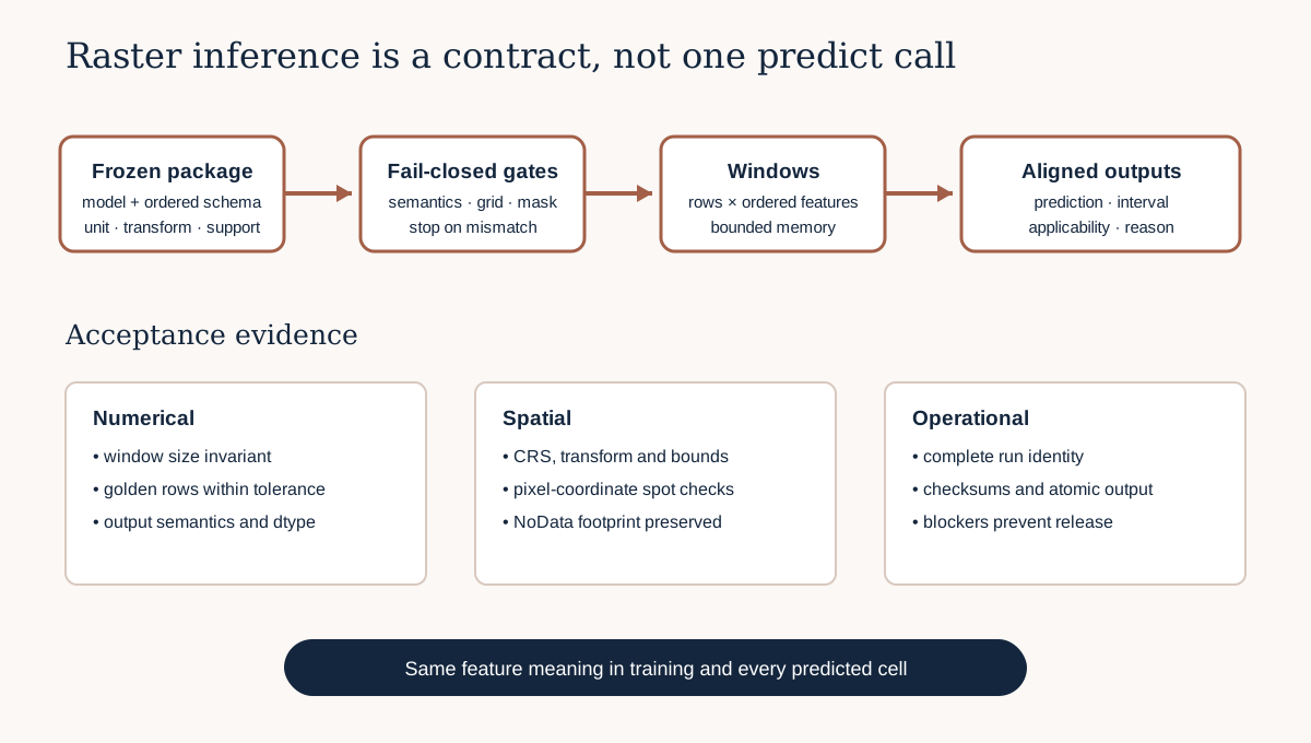
Each window uses the same feature names, order, transformation, mask logic and model. Windowing is a computational partition only. It must not redefine the scientific prediction unit or fit any transformation from the deployment scene.

5. Worked example — validate the prediction schema before reading pixels

Predict before running

The training and prediction schemas contain the same feature names, but the prediction stack records uav_height_p95 in metres rather than centimetres. Should the code reorder and proceed, warn and proceed, or stop?

def validate_prediction_schema(actual, expected):
    actual_names = [item["name"] for item in actual]
    expected_names = [item["name"] for item in expected]
    if actual_names != expected_names:
        raise ValueError(f"Feature order mismatch: {actual_names}")
    for observed, required in zip(actual, expected):
        for field in ("unit", "transform", "support", "version"):
            if observed[field] != required[field]:
                raise ValueError(f"{observed['name']} changed {field}")
    return True

Code walkthrough

1. The function receives the observed deployment schema and the model's saved requirement.
2. Names are extracted in their actual order.
3. Exact list equality prevents silent reordering and missing or extra features.
4. zip is safe only after equal ordered names have been established.
5. Unit comparison catches centimetre–metre errors.
6. Transformation comparison catches different scaling, index or composite rules.
7. Support comparison protects the ecological and spatial meaning of each value.
8. Version comparison detects an unreviewed source or preprocessing change.
9. A mismatch raises an exception before any map is created.

In production, validate additional fields such as dtype, valid range, temporal window, resampling and hash. The function demonstrates a fail-closed principle rather than a complete schema language.

Diagnostic check

Create three deliberately wrong schemas: reorder two features, change one unit and update one source version. Confirm that each fails with a specific message. Then compare the validated names with the DataFrame columns passed to XGBoost while validate_features=True. The application-level schema protects meaning; XGBoost's feature validation provides an additional name/order check, not a replacement for unit and support metadata.

Check your understandingA prediction stack has the correct band names and order, but its NDVI uses a different seasonal composite. May inference proceed?

Choose one answer

No; temporal transformation is part of the feature schemaYes; names and order are enoughOnly when the raster dimensions are unchanged

Check answer

6. Construct the valid prediction mask

For each window, a cell is eligible only when:

• it lies inside the declared prediction domain;
• every required feature is present after the frozen preprocessing;
• source QA flags permit use;
• numeric values are finite and within hard physical or encoding constraints;
• the grid cell is not source NoData;
• any required temporal-completeness rule passes.

Combine required masks with logical AND. Preserve separate reason flags for missing input, cloud/shadow, invalid geometry, temporal insufficiency and other upstream failures. Do not call invalid input “outside applicability”; applicability is evaluated only for feature vectors that exist.

Optional features require a model trained to handle their documented absence. Dropping a missing column from the prediction matrix changes the model schema and is not permitted.

Check your understandingA cell has all required predictor values but lies outside applicability. What should the output preserve?

Choose one answer

A withheld state distinct from NoDataNoData because every unusable value means missing inputA supported state when the interval is narrow

Check answer

7. Convert a raster window into model rows

Assume a stack with shape (features, rows, columns). Move the feature axis last and reshape to (rows × columns, features). Apply the flattened valid mask, predict only eligible rows, then place results back into a window-sized array initialized to output NoData.

Keep these contracts explicit:

• feature_stack[i] corresponds exactly to feature_order[i];
• reshape order used for features, mask and outputs is identical;
• model input uses the fitted dtype or a validated compatible dtype;
• no scaler or imputer is fitted on prediction windows;
• output row/column positions remain stable after filtering;
• uncertainty and applicability functions receive the same eligible feature rows.

Write a unit test with a tiny 2 × 3 grid whose expected output can be calculated by hand. A full-scene visual check cannot replace index-level tests.

8. Windowed inference

Window size is an operational parameter chosen from memory, I/O and model throughput. It is not a modelling hyperparameter and should not alter values. Iterate over the reference grid's block windows or a declared tiling scheme:

1. read corresponding windows from every required feature;
2. verify window offsets and shapes;
3. build validity and reason masks;
4. construct the ordered feature matrix;
5. predict point, bounds and applicability for valid rows;
6. apply the frozen release policy;
7. write each output to the identical destination window;
8. record counts, minima, maxima and errors;
9. continue only when all writes succeed.

Use a temporary destination or incomplete marker. Publish final filenames only after all windows and checks pass. A partially written GeoTIFF with a correct header is not a valid product.

9. Regression, class and probability outputs

Different outputs need different contracts:

• regression: floating dtype, target unit status, meaningful range and floating NoData;
• class: integer codes, class dictionary, reserved NoData distinct from any valid class;
• probability: floating values in [0, 1], declared positive class or class-band order, calibration version and floating NoData;
• interval bounds/width: floating target units, nominal level, method and calibration version;
• applicability/release state: categorical codes with machine-readable meanings and reasons.

Do not cast regression predictions to an integer for file size. Do not store probability as 0–100 without documenting scale. Compression and tiling may change storage, never semantic values.

10. Validate prediction values without changing them

Operational QA should identify:

• non-finite predictions;
• values outside documented physical or training-informed review ranges;
• lower bounds above upper bounds;
• probabilities outside [0,1];
• class codes absent from the dictionary;
• impossible released values at invalid-input cells;
• suspicious constant windows or seams;
• prediction count disagreement with the valid mask;
• applicability or uncertainty layers missing where a prediction exists.

A review range is not permission to clip. Preserve the original value, assign a reason and follow the release policy. Any transformation applied after prediction becomes part of the evaluated procedure and must have been frozen before operational use.

11. Spatial acceptance tests

For every output, compare against the reference grid:

• CRS, transform, width, height and bounds;
• pixel size and orientation;
• block layout and window coverage;
• NoData and mask consistency;
• stable checksum or metadata digest;
• known control-cell positions and expected values;
• coverage of every window exactly once;
• absence of overlaps, gaps and one-pixel shifts.

Create a seam test by predicting the same small region with one full window and several subwindows. Values must agree within declared numeric tolerance. If they do not, investigate stateful preprocessing, edge context or indexing.

Check your understandingWhat should change when a raster is predicted in smaller windows?

Choose one answer

Memory demand, but not valid-cell predictions or spatial placementFeature orderThe model's target unit

Check answer

12. Run metadata and provenance

inference_run.json should record:

• run ID, start/end time and status;
• model, feature schema, interval and applicability versions;
• code commit and environment lock;
• input asset IDs, checksums or immutable versions;
• reference grid and prediction-domain IDs;
• window dimensions and total/completed windows;
• valid, NoData, review and withheld counts;
• output paths, dtypes, NoData and checksums;
• warnings, failures and operator;
• acceptance-test results.

The log must be written even when the run fails. A failure record prevents an abandoned output from being mistaken for an approved release.

13. Model clinic — the map looks correct

A national prediction raster has the expected colours, but feature bands were sorted alphabetically instead of using the training order.

• Problem: the model received valid numbers with incorrect meanings.
• Evidence: saved feature order, actual stack order, control-cell feature vectors and model input columns.
• Consequence: every prediction may be wrong without a software exception.
• Fix: fail on ordered-schema mismatch, rebuild from immutable inputs and rerun all acceptance tests. Do not rename the output as corrected evidence.

14. Common mistakes

Fitting scaling per window

Why beginners make it: standardization code is nearby. Recognition: each tile has mean zero. Fix: load the fitted training transformation. Consequence: identical values receive different model inputs across windows.

Treating NaN as a model feature

Why: XGBoost can route missing values. Recognition: source NoData is sent into a model that was not trained for that absence mechanism. Fix: enforce the frozen missingness contract. Consequence: missing imagery produces unvalidated predictions.

Reordering features automatically

Why: matching by name seems helpful. Recognition: operational code silently repairs stack order. Fix: fail, record and rebuild the stack. Consequence: upstream contract failure is hidden.

Publishing after the last write

Why: processing completed. Recognition: no acceptance phase exists. Fix: validate geometry, counts, values, evidence layers and checksums before promotion. Consequence: incomplete or shifted outputs become official.

Using window count as ecological sample size

Why: the run has many chunks. Recognition: performance language references millions of pixels. Fix: keep reference-observation and validation evidence separate. Consequence: computational scale is confused with scientific evidence.

15. Guided practice — build a fail-closed spatial predictor

1. Add ## Lesson 3.26 checkpoint to the cumulative notebook.
2. Load the serialized model and its immutable metadata.
3. Load expected and actual feature schemas.
4. Validate order, unit, transform, support, temporal rule, dtype and version.
5. Validate every predictor against the reference grid.
6. Create a temporary output group and failed-run marker.
7. Test the reshape/write logic on a hand-checkable 2 × 3 grid.
8. Iterate over windows from the reference raster.
9. Read features in saved order and create reason-specific validity masks.
10. Predict point, bounds and applicability only for eligible rows.
11. Apply the frozen release policy without clipping.
12. Write all aligned output windows and collect counts.
13. Compare full-window and subwindow predictions on a control region.
14. Validate output geometry, dtype, NoData, ranges, relationships and coverage.
15. Write run metadata and checksums.
16. Promote temporary outputs only after every gate passes.
17. Simulate a failed window and confirm the package cannot be released.

16. Independent challenge — schema-compatible but scientifically different

The replacement stack has identical names, order, shape and dtype. Its sentinel2_ndvi is a monthly maximum rather than the training-time nearest-date composite. Extend the schema validator and run policy to detect the difference. Explain why numeric correlation between the products cannot authorise substitution without fresh evaluation.

17. Scientific interpretation

Raster inference does not create new accuracy evidence. It applies a previously evaluated procedure to many prediction units while preserving semantics and recording where use is supported. The output is defensible only when model, features, grid, masks, uncertainty, applicability and run metadata remain linked.

Windowing makes computation manageable; it cannot make unsupported geographic transfer valid. Chapter 5 applicability and Chapter 6 uncertainty gates must accompany the point raster at operational scale.

18. Submission

Submit:

• executed Lesson 3.26 notebook checkpoint;
• prediction_schema.json and validator tests with deliberate failures;
• spatial_prediction_pipeline.py with window, mask, reshape, predict, write and failure handling;
• aligned point, interval, applicability and release-state teaching outputs;
• inference_run.json with counts, versions, warnings and acceptance results;
• a control-grid and seam-test report.

The submission fails if it silently reorders features, fits transformations on deployment, predicts invalid inputs, publishes partial output, omits evidence layers or treats pixel count as validation evidence.

19. Portfolio artifact

Operational Monitoring Pipeline — Spatial Prediction Component

This component converts the fixed Prediction Evidence Package into a repeatable, fail-closed raster inference run. Lesson 3.27 evaluates which part of the workflow can be implemented natively in Google Earth Engine.

Reflection

1. Which schema fields protect scientific meaning beyond feature names?
2. Why must window size leave predictions unchanged?
3. What is the difference between NoData and withheld use?
4. Which acceptance test would catch a one-pixel shift?
5. What evidence is still unchanged after predicting ten million cells?

20. Core references

• XGBoost 3.3 Python API, feature validation and model IO
• Rasterio windowed reading and writing
• OGC Cloud Optimized GeoTIFF standard

Further advanced reading

• XGBoost prediction API
• GDAL raster data model

21. Tested software versions

The modelling contracts and tests target Python 3.12.13, NumPy 2.4.2, pandas 2.2.3, scikit-learn 1.9.0 and XGBoost 3.3.0. Raster implementation must retain the tested Rasterio/GDAL environment recorded by Module 2. The synthetic Chapter 7 pack supplies control metadata, not real prediction rasters.

Functional-landscape bridge

Aligned UAV predictors → fitted model → trait prediction surface can support later analysis of trait heterogeneity or functional diversity. Richness, CWM and functional diversity answer different questions; AGB is biomass/productivity and is not one of the traits in the project’s composite functional-diversity metric. Review the observed–derived–modelled lineage.