Conformal Prediction and Empirical Coverage

1. Problem — nominal coverage needs calibration evidence

Learning outcome

By the end of this lesson, you will be able to explain split conformal prediction at an applied scientific level; separate model-training, calibration and assessment roles; calculate absolute-residual nonconformity scores and the finite-sample conformal quantile; build symmetric prediction intervals; evaluate marginal and structured empirical coverage; diagnose violations of exchangeability caused by spatial dependence or temporal shift; and state coverage claims without implying conditional certainty.

• Lesson type: Structured Split-conformal Coverage Laboratory
• Estimated time: 250–340 minutes
• Prerequisites: Lessons 3.9–3.12, 3.17, 3.21–3.23
• Portfolio outputs: conformal_predictions.csv, CONFORMAL_COVERAGE_REPORT.md, coverage_stress_test.csv, calibration_roles.json and the Lesson 3.24 notebook checkpoint

Why this matters

A quantile model may target an 80% interval and achieve only 65% coverage on unseen meadows. Conformal prediction adds a calibration step that uses held-out prediction errors to set or adjust interval width. Under exchangeability and the specified procedure, split conformal offers a finite-sample marginal coverage result without assuming normally distributed residuals or a correct parametric model.

Earth Observation data make the assumption difficult. Nearby pixels share processes, sites differ, and future acquisitions can shift. The correct educational response is neither to dismiss conformal methods nor to advertise distribution-free coverage without conditions. We must define the exchangeable unit, preserve groups and time, and test coverage where the model is intended to transfer.

Core lesson: conformal coverage comes from the calibration design and its assumptions, not from attaching the word “conformal” to an interval.

Mental model

proper training → fixed predictor model
calibration labels → nonconformity scores → finite-sample quantile
fixed model + quantile → assessment intervals
assessment labels → empirical coverage, width and transfer diagnosis

Each arrow has a permitted data role. If an assessment label moves backward into calibration, the reported coverage no longer evaluates the frozen procedure.

2. Scientific context — three evidence roles

The Environmental Monitoring Project now divides permitted development evidence into:

• proper training: fit preprocessing and the point or quantile model;
• calibration: observe errors from the already fitted model and construct the interval rule;
• assessment: evaluate the frozen model-plus-calibration procedure without changing it.

The sealed final test remains a fourth role and is still unopened. Site, spatial block and acquisition period stay attached to every observation. Randomly scattering neighbouring rows across these roles would contradict the intended new-site or future-time claim.

3. Concept — nonconformity measures surprise

For a fitted point model $\hat{f}$, a simple regression nonconformity score is the absolute calibration residual:

$$s_i = |y_i - \hat{f}(x_i)|$$

Large scores indicate calibration outcomes that conform poorly to the fitted prediction. For desired miscoverage $\alpha$, split conformal selects a high empirical score quantile $\hat{q}$ and returns:

$$C(x) = [\hat{f}(x)-\hat{q},\ \hat{f}(x)+\hat{q}]$$

This symmetric interval has constant half-width. It is an excellent mechanism to understand before moving to adaptive scores or conformalized quantile regression.

4. Visual explanation — training, calibration and assessment never swap roles

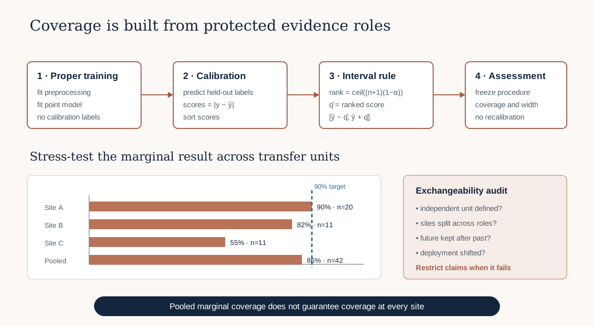
The workflow has two protections. First, calibration labels do not fit the point model. Second, assessment labels do not choose $\hat{q}$. The site-level panel reminds us that pooled marginal coverage can conceal failed transfer.

5. Worked example — calculate a finite-sample split-conformal interval

Predict before running

With 19 calibration scores and a 90% target, should NumPy's ordinary interpolated 90th percentile be used without adjustment? What rank protects the finite calibration sample?

import numpy as np

calibration_prediction = model.predict(X_calibration[feature_order])
scores = np.abs(y_calibration - calibration_prediction)
alpha = 0.10
n = len(scores)
rank = min(n, int(np.ceil((n + 1) * (1 - alpha))))
q_hat = np.sort(scores)[rank - 1]

test_prediction = model.predict(X_assessment[feature_order])
lower = test_prediction - q_hat
upper = test_prediction + q_hat
covered = (y_assessment >= lower) & (y_assessment <= upper)

Code walkthrough

1. The already fitted model predicts the calibration rows without having trained on their labels.
2. Absolute residuals become nonconformity scores.
3. alpha=0.10 targets 90% marginal coverage.
4. n is the number of valid calibration scores—not the number of pixels generated from them.
5. The rank uses $\lceil(n+1)(1-\alpha)\rceil$, capped at the available sample size.
6. Sorting and choosing rank - 1 implements a conservative empirical order statistic without linear interpolation.
7. The frozen point model predicts untouched assessment observations.
8. q_hat expands each point symmetrically.
9. The Boolean vector records empirical coverage after outcomes are revealed.

If the requested rank exceeds the calibration size, the desired finite-sample level cannot be represented by a more extreme observed score. The cap produces the widest score-supported interval, but the small calibration count must remain explicit.

Diagnostic check

Print the sorted calibration scores with their observation ID, site and spatial block. Confirm that the selected score is at the recorded rank and that ties are handled deterministically. Then verify that calibration groups are absent from proper training and that assessment groups are absent from both. A numerical q_hat without this lineage is not a conformal evidence record.

Create a second diagnostic in which scores are coloured by site. If the highest scores come from one environmental regime, a global symmetric width may hide conditional failure even when its pooled marginal coverage is acceptable.

6. Why the finite-sample correction matters

An interpolated percentile can fall between observed scores and understate the conformal order statistic. Conformal algorithms often express the adjusted quantile as:

$$\operatorname{Quantile}_{\lceil(n+1)(1-\alpha)\rceil/n}(s_1,\ldots,s_n)$$

using a “higher” order-statistic rule. The explicit rank in the worked example is easy to audit across software versions. Record the formula, alpha, score definition, number of scores and tie behaviour in metadata.

7. What the coverage statement means

Under exchangeability of calibration and future examples, split conformal targets marginal coverage over repetitions of the complete data-generating process:

$$P\{Y_{new} \in C(X_{new})\} \ge 1-\alpha$$

It does not generally guarantee:

• 90% coverage for every site, habitat, predictor value or individual cell;
• a 90% posterior probability that the already produced interval contains its fixed target;
• validity after sensor, season or management-regime shift;
• joint coverage of every pixel in an entire raster;
• coverage after selecting alpha or the score on assessment labels.

Report the target as a property of the procedure under assumptions, then show empirical protected coverage with binomial uncertainty and group counts.

Check your understandingA nominal 90% interval covers 90% of pooled rows but only 55% at one held-out site. What is the conclusion?

Choose one answer

Pooled marginal coverage conceals poor transfer coverage and the claim must be restrictedThe method is valid everywhere because pooled coverage is 90%The failed site should be removed

Check answer

8. Exchangeability in spatial and temporal data

Exchangeability means the joint distribution is unchanged by reordering the examples relevant to the conformal argument. Independent and identically distributed sampling is sufficient but stronger than exchangeability. Spatial autocorrelation, hierarchical sampling and temporal drift can invalidate a naive row-level assumption.

For the Academy project:

• define whether the intended prediction is a new plot within represented sites, a new site or a future acquisition;
• treat the corresponding independent unit—not every derivative pixel—as the primary evidence unit;
• create calibration and assessment partitions that preserve sites, blocks or temporal direction;
• report how few genuinely independent units remain;
• examine empirical coverage by held-out site, distance, year and applicability;
• treat structured splitting as an alignment and stress test, not a magical proof that the standard guarantee now holds;
• use methods designed for dependence only when their assumptions and implementation are understood and tested.

Recent research extends conformal ideas to some non-exchangeable settings, often with additional assumptions or coverage penalties. This core lesson does not promise those results from ordinary split conformal.

Check your understandingWhy is ordinary split conformal delicate for spatial or temporal EO data?

Choose one answer

Dependence and distribution shift can make calibration and deployment scores non-exchangeableCoordinates make quantiles undefinedConformal prediction requires a linear model

Check answer

9. Calibration is part of model development

Choosing the score, alpha, grouping, local scaling or adaptive method changes the prediction procedure. These decisions belong inside development evidence. A nested evaluation can work as follows:

1. outer assessment groups remain untouched;
2. outer development groups are divided into proper training and calibration according to a preregistered rule;
3. the point model and score rule are fitted;
4. the interval procedure predicts the outer assessment group once;
5. coverage and width are stored;
6. the process repeats for every outer fold;
7. model and interval choices are frozen before final-test use.

The resulting fold estimates describe the complete model-plus-calibration procedure. Never calibrate on the same outer labels whose coverage you report.

Check your understandingWhich labels may calculate split-conformal nonconformity scores?

Choose one answer

A calibration partition kept separate from model fitting and final assessmentThe final assessment labelsEvery prediction-grid cell

Check answer

10. From symmetric conformal to adaptive intervals

Constant-width intervals are transparent but cannot respond to heteroscedasticity. Two principled extensions are:

• normalised scores: divide absolute residuals by a development-fitted scale estimate, then multiply the conformal quantile by the new unit's scale;
• conformalized quantile regression (CQR): begin with lower and upper quantile predictions, calculate calibration scores such as $\max(l_i-y_i, y_i-u_i)$, and expand both bounds by the calibrated quantile.

CQR can retain predictor-dependent width while correcting marginal coverage. It does not remove exchangeability assumptions or applicability limits. Treat it as an advanced extension after the symmetric procedure is fully audited.

11. Evaluate coverage as structured evidence

Create a table with one row per protected observation and columns for observation ID, site, block, date, target, point, lower, upper, width, covered, miss direction and applicability state. Then report:

• pooled coverage and count;
• fold coverage, width and independent-group count;
• site and acquisition-period coverage where counts permit;
• coverage inside supported, review and outside-applicability states;
• coverage across interval-width bands;
• lower and upper miss counts;
• calibration-score distribution and chosen order statistic.

Use a binomial confidence interval to communicate sampling variability in empirical coverage, while remembering that ordinary binomial calculations also assume independent Bernoulli trials. When observations are clustered, counts and group-level results are essential.

12. Model clinic — pooled coverage passes

The 90% conformal procedure covers 45 of 50 assessment rows. At one held-out meadow it covers 6 of 11.

• Problem: pooled coverage meets the numerical target while a transfer site fails.
• Evidence: site identity, score distribution, interval width, applicability and predictor shift.
• Consequence: a universal “90% coverage” claim would misrepresent the intended new-site use.
• Fix: restrict the claim, investigate exchangeability and support, and collect calibration evidence relevant to that destination. Do not delete the failed site or recalibrate on its assessment labels.

13. Common mistakes

Training the model on calibration labels

Why beginners make it: more data improves the point model. Recognition: the fitted model has seen every score's outcome. Fix: preserve proper-training and calibration roles. Consequence: scores are too small and intervals undercover.

Using ordinary interpolated percentiles

Why: default quantiles are convenient. Recognition: selected q_hat is between score values without a documented method. Fix: implement the finite-sample order statistic. Consequence: the intended coverage correction is lost.

Recalibrating after assessment failure

Why: widening reaches the target. Recognition: outer labels change q_hat. Fix: treat failure as assessment evidence and revise on fresh development data. Consequence: assessment is no longer independent.

Calling the method assumption-free

Why: “distribution-free” is shortened incorrectly. Recognition: exchangeability and transfer conditions are absent. Fix: state what distributional form is avoided and which sampling assumption remains. Consequence: geospatial dependence is hidden.

Treating every pixel as an independent coverage trial

Why: rasters provide millions of cells. Recognition: coverage precision is based on pixel count from a few field supports. Fix: respect independent target observations and spatial support. Consequence: uncertainty about coverage is drastically understated.

14. Guided practice — construct and stress-test split conformal intervals

1. Add ## Lesson 3.24 checkpoint to the cumulative notebook.
2. State the desired coverage, destination claim and exchangeable unit.
3. Load the frozen outer-fold registry.
4. Within each outer development role, separate proper-training and calibration groups without spatial overlap.
5. Fit preprocessing and the point model on proper training only.
6. Predict calibration outcomes and calculate absolute-residual scores.
7. Record score count, alpha, adjusted rank and q_hat.
8. Freeze the interval rule.
9. Predict the untouched outer assessment group.
10. Save bounds, width, covered state and miss direction.
11. Repeat without allowing outer labels into model or calibration decisions.
12. Calculate pooled, fold and site coverage with counts.
13. Compare width and coverage across applicability states.
14. Identify evidence relevant to exchangeability and transfer.
15. Compare symmetric conformal with the already frozen quantile interval without tuning either on outer evidence.
16. Write a precise coverage claim and at least three limitations.
17. Keep final-test data sealed.

15. Independent challenge — calibration unit redesign

The available calibration set contains 120 rows but only four independent sites; 90 rows come from one site. Compare row-level random calibration, site-preserving calibration and a leave-one-site assessment. Explain what each can support, how the effective evidence changes and why a large row count does not solve weak site replication. Propose new sampling rather than inventing a guarantee.

16. Scientific interpretation

Split conformal prediction converts observed calibration surprises into an auditable interval rule. Its strength is that the rule can be inspected, reproduced and empirically tested without specifying a normal residual distribution. Its limit is equally important: coverage belongs to a population and sampling relation, not to software syntax.

For spatial EO, credible practice combines a declared exchangeable unit, structured separation, protected coverage assessment, applicability, group diagnostics and transparent limitations. Coverage that fails at a destination is evidence to restrict or improve the procedure—not an invitation to tune on that destination's test labels.

17. Submission

Submit:

• the executed Lesson 3.24 notebook checkpoint;
• calibration_roles.json identifying proper-training, calibration, assessment and sealed-test roles;
• conformal_predictions.csv with point, bounds, score-derived width, coverage and groups;
• coverage_stress_test.csv with pooled, fold, site and applicability summaries plus counts;
• CONFORMAL_COVERAGE_REPORT.md stating score, formula, alpha, rank, empirical results, exchangeability analysis and bounded claim;
• one accessible coverage figure and text alternative.

The submission fails if model fitting uses calibration labels, calibration uses assessment labels, the quantile rule is undocumented, row counts masquerade as independent sites or the report claims universal or conditional coverage from pooled marginal evidence.

Reflection

1. What is the exchangeable unit for your intended destination?
2. Which label roles must never overlap?
3. Why is the finite-sample conformal quantile not an ordinary interpolated percentile?
4. What can pooled marginal coverage conceal?
5. Which new calibration evidence would most strengthen the transfer claim?

18. Portfolio artifact

Prediction Evidence Package — Conformal Coverage Report

This component adds a calibrated interval procedure, empirical structured coverage and an exchangeability audit. Lesson 3.25 will turn point, interval and applicability evidence into aligned map products and a release policy.

19. Core references

• Angelopoulos and Bates (2023), Conformal Prediction: A Gentle Introduction
• Romano, Patterson and Candès (2019), conformalized quantile regression
• Oliveira et al. (2024), split conformal prediction and non-exchangeable data

Further advanced reading

• Vovk, Gammerman and Shafer (2005), Algorithmic Learning in a Random World
• Tibshirani et al. (2019), conformal prediction under covariate shift

20. Tested software versions and professional standard

The explicit finite-sample order statistic was tested with Python 3.12.13 and NumPy 2.4.2; tabular evaluation uses pandas 2.2.3 and the fixed point model uses the project's scikit-learn 1.9.0 / XGBoost 3.3.0 environment. A professional conformal report publishes data roles, score, order statistic, alpha, sample and group counts, empirical coverage, width, structured failures, applicability and exchangeability limitations.