What Does a Useful Model Need to Beat?

1. Problem — complexity is not a reference point

Learning outcome

By the end of this lesson, you will be able to define regression and classification baselines, fit them using training evidence only, compare a candidate on identical held-out observations, calculate error skill relative to a declared baseline, diagnose underfitting, and write a baseline_report.md that states what a future model must beat.

• Lesson type: Baseline and Skill Laboratory
• Estimated time: 150–210 minutes
• Prerequisites: Lessons 3.1–3.4; Module 1 summary statistics, pandas and plotting; Module 2 sampling, grouped evidence and spatial support
• Portfolio output: baseline_report.md

Why this matters

A complex model can produce plausible predictions and attractive maps while adding no useful information. If a candidate predicting vegetation height has a mean absolute error of 12 cm, is that good? The number is uninterpretable until it is compared with a rule that uses less information. A training-fold mean might already produce 10 cm error. A transparent linear model may produce 7 cm. In that case, the complex candidate has not earned its operational cost.

Baselines are not deliberately bad models. They are scientific controls. Each answers a different question:

• Does the candidate beat ignoring all predictors?
• Does it beat using the typical training target?
• Does it beat a transparent relationship with one or a few predeclared predictors?
• Does it beat the current operational rule or previous model?

Core lesson: model performance means improvement over a relevant comparator on the same independent cases—not a large-looking score in isolation.

Mental model

Think of a ladder with increasing information and flexibility:

1. naive constant rule — uses no predictors;
2. simple scientific baseline — uses a transparent, predeclared relationship;
3. candidate model — uses greater flexibility and complexity.

Every rung must be trained on the same permitted development evidence and evaluated on the same validation observations. If a complex model does not clear a lower rung consistently, the lower rung remains the stronger professional choice.

2. Scientific context — a synthetic height-prediction experiment

Continue the Environmental Monitoring Project using the Chapter 2 synthetic coastal-meadow fixture. Its response field, vegetation_height_cm, has a supplied teaching definition and unit. Its EO-style predictors include vegetation indices, a UAV height percentile and texture. The values are generated for instruction; they are not measurements from the published Baltic coastal plant-traits record.

The experiment plan from Lesson 3.4 declares:

• prediction target: synthetic vegetation_height_cm;
• prediction unit: one synthetic plot-level modelling observation;
• Chapter 2 validation split: the rows labelled validation in the saved registry;
• final test: rows labelled sealed, which must not be opened;
• primary Chapter 2 metric: MAE in centimetres;
• secondary diagnostic: RMSE in centimetres;
• first complex candidate: an untuned XGBoost regressor in Lesson 3.8.

Chapter 2 does not yet claim new-site or new-region transfer. Chapter 3 will challenge the validation design. For now, the fixed development split lets you compare mechanisms without silently changing cases.

3. Concept — what a baseline represents

Regression baselines

For a continuous target, useful starting comparators include:

Training mean. Predict the arithmetic mean of the training targets for every validation observation. This minimises squared error among constant predictions, which makes it a natural comparator when RMSE or squared loss matters.

Training median. Predict the training median for every validation observation. The median is less influenced by extreme target values and is a natural constant comparator for absolute error. It is not automatically superior; its relevance depends on the declared metric and target distribution.

Simple linear model. Use one or a small predeclared set of scientifically interpretable predictors. This asks whether an approximately linear relationship already captures the usable signal. It is a stronger comparator than a constant rule because it uses features.

Classification baselines

For a categorical target, a comparable ladder might include:

• most frequent class — always predicts the majority training class;
• class-prior probability — returns the training class frequencies as probabilities;
• simple logistic model or shallow tree — uses a transparent feature relationship.

A majority baseline can have high accuracy when a habitat class is rare while never identifying that habitat. Lesson 3.16 will treat class imbalance, thresholds and error costs properly. At this point, record class-wise outcomes instead of accepting accuracy alone.

A baseline is fitted

The training mean and majority class depend on target values, so they are fitted estimators. Calculate them from the training fold only. If validation targets influence the constant, the comparison leaks held-out information even though no machine-learning algorithm was used.

Check your understandingWhich observations may determine a mean baseline used to score one validation fold?

Choose one answer

Only the corresponding training observationsTraining and validation observations togetherThe final test observations only

Check answer

4. Visual explanation — the baseline ladder and evaluation firewall

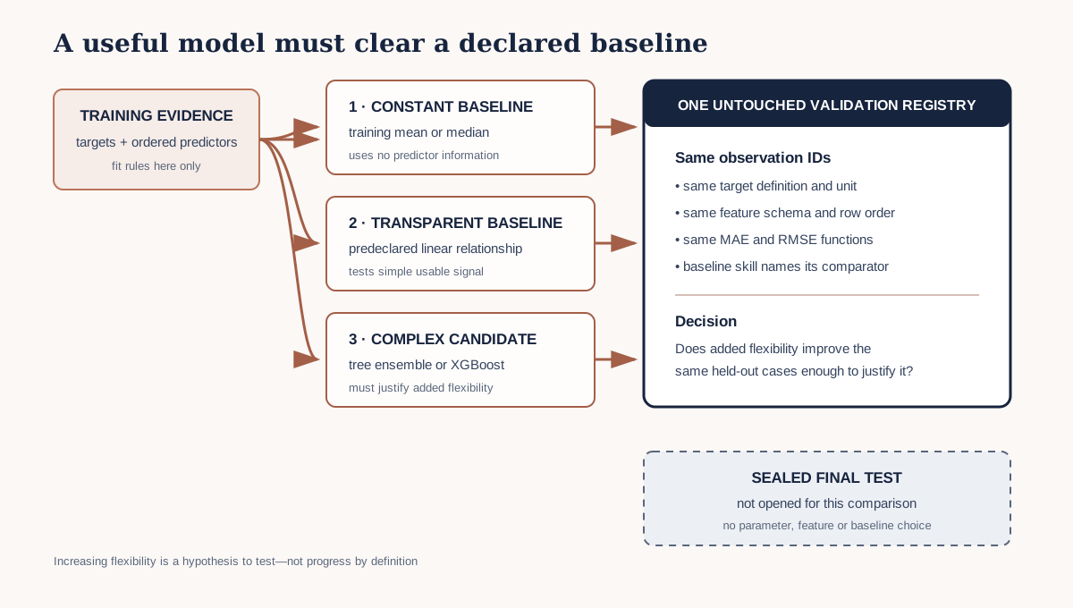
The vertical order represents increasing flexibility, not guaranteed improvement. The horizontal firewall is the crucial design feature: validation targets score the predictions but do not determine the training mean, regression coefficients or candidate parameters. The sealed final test is outside the Chapter 2 comparison.

5. Metrics and model skill

Let observed targets be $y_i$, predictions be $\hat{y}_i$, and $n$ be the number of validation observations.

Mean absolute error reports the average absolute miss:

$$MAE = \frac{1}{n}\sum_{i=1}^{n}|y_i-\hat{y}_i|$$

Its unit is the target unit. An MAE of 6 cm means the validation predictions were about 6 cm from their targets on average, without indicating direction.

Root mean squared error gives larger errors more influence:

$$RMSE = \sqrt{\frac{1}{n}\sum_{i=1}^{n}(y_i-\hat{y}_i)^2}$$

It also retains the target unit. A much larger RMSE than MAE suggests some errors are relatively large, but the two metrics do not identify which sites or conditions caused them.

For an error metric where lower is better, define skill against the baseline as:

$$Skill = 1 - \frac{Error_{candidate}}{Error_{baseline}}$$

• 1 would mean zero candidate error;
• 0 means no improvement over the baseline;
• a value between 0 and 1 means improvement;
• a negative value means the candidate is worse.

Name the error metric whenever reporting skill. “Skill = 0.3” is incomplete; “MAE skill relative to the training-mean baseline = 0.3” is reviewable.

Check your understandingA candidate has higher validation MAE than the predeclared mean baseline. What does this show?

Choose one answer

The candidate has negative error skill for that comparisonThe candidate is useful because it is more complexThe baseline must be removed from the report

Check answer

6. Worked example — fit the mean baseline behind the split

Predict before running

Suppose the training target mean is 31.4 cm. Predict whether every validation prediction will equal 31.4. If the validation targets average 36 cm, should that change the fitted baseline? Explain before running.

import pandas as pd
from sklearn.dummy import DummyRegressor
from sklearn.metrics import mean_absolute_error, root_mean_squared_error

data = pd.read_csv("data/baseline_modelling_data.csv")
train = data.loc[data["chapter2_split"] == "train"]
validation = data.loc[data["chapter2_split"] == "validation"]
features = ["sentinel2_ndvi", "uav_height_p95"]

mean_model = DummyRegressor(strategy="mean")
mean_model.fit(train[features], train["vegetation_height_cm"])
predictions = mean_model.predict(validation[features])

mae = mean_absolute_error(validation["vegetation_height_cm"], predictions)
rmse = root_mean_squared_error(validation["vegetation_height_cm"], predictions)
print(f"Mean baseline: MAE={mae:.2f} cm; RMSE={rmse:.2f} cm")

Code walkthrough

1. pandas loads the saved teaching table.
2. DummyRegressor provides an estimator interface for simple prediction rules that ignore features.
3. The metric functions score continuous predictions; both return values in centimetres here.
4. train selects only rows authorised for fitting.
5. validation selects the fixed Chapter 2 comparison cases.
6. features is present because the estimator interface expects an input matrix, although the mean rule ignores feature values.
7. strategy="mean" declares the exact rule rather than constructing an unexplained constant manually.
8. .fit(...) calculates the constant from training targets only.
9. .predict(...) repeats that constant once for each validation row.
10. MAE and RMSE compare predictions with validation targets after fitting is complete.
11. The final line reports metric names, values and target units.

Diagnostic check

Run:

assert len(predictions) == len(validation)
assert len(set(predictions.round(10))) == 1
assert not data.loc[data["chapter2_split"] == "sealed"].index.isin(train.index).any()

The first check protects row alignment. The second confirms this estimator is truly constant. The third documents that sealed rows were not included in the training object. It does not prove the whole notebook avoided them; record cell inputs and row counts in the report.

7. Build the comparator set

Repeat the identical fitting and evaluation sequence for:

1. DummyRegressor(strategy="median");
2. a LinearRegression using only uav_height_p95;
3. optionally, a predeclared two-predictor linear model if the experiment plan names it.

Do not choose the simple model after examining many predictors and reporting only the best. That would convert the “baseline” into an unreported feature search. The baseline should be declared because it represents existing knowledge or a minimum plausible decision rule.

Create one tidy comparison table:

model	uses predictors	fit rows	score rows	MAE cm	RMSE cm	MAE skill vs mean
training mean	no	…	…	…	…	0.000
training median	no	…	…	…	…	…
linear UAV height	yes	…	…	…	…	…

Keep the target unit in the column names or metadata. Include a split_version and dataset checksum so the table cannot be separated from its evidence design.

8. Bias–variance intuition without slogans

Bias here describes systematic limitations in the model’s expected predictions. A constant baseline cannot respond to vegetation structure, so it is strongly constrained and likely underfits.

Variance describes sensitivity to the particular training sample. A highly flexible tree may follow small training peculiarities and change substantially when the sample changes.

The terms are properties of repeated sampling and model behaviour, not labels you can prove from one train/validation result. Use them as a diagnostic mental model:

• similar weak training and validation performance suggests insufficient useful structure or strong underfitting;
• excellent training but weak validation performance suggests excessive sample-specific fit, leakage or domain mismatch;
• stable improvement over baselines across appropriate folds is stronger evidence of useful signal.

A simple model can have low variance and high bias. A complex model can reduce bias while increasing variance. The goal is not the most complex model; it is credible generalisation for the intended domain.

Check your understandingWhy keep a simple linear baseline alongside a constant baseline?

Choose one answer

It tests whether a transparent relationship captures most usable signalIt guarantees the final model is causalIt removes the need for structured validation

Check answer

9. Model clinic — impressive R² without a baseline report

Situation: a team reports validation $R^2=0.72$ for vegetation height and calls the model highly useful. No baseline error, target range, validation case count or site distribution is reported.

Question	Diagnosis
problem	one dimensionless score is presented without comparators or operational scale
evidence needed	mean/median and transparent-model errors on identical rows, units, fold identities, target distribution and subgroup diagnostics
consequence	readers cannot tell whether errors are small enough for the intended decision or whether a simpler model performs similarly
fix	restore the predeclared comparator ladder and report absolute errors, skill and validation scope

R² is not rejected; it is simply insufficient. Lesson 3.17 will examine it alongside MAE, RMSE, bias, residual plots and fold variability.

10. Common mistakes and recovery

Calculating the baseline from all targets

• Why it happens: the mean looks like descriptive preprocessing rather than fitting.
• How to detect it: the baseline constant equals the full-table mean, not the training-fold mean.
• How to prevent it: implement the baseline through the same fit/predict boundary as every model.
• Consequence: validation information improves the reference prediction.

Choosing a deliberately weak baseline

• Why it happens: beating it makes the candidate look impressive.
• How to detect it: a relevant existing rule or simple feature-aware model is omitted.
• How to prevent it: state what each baseline represents before fitting.
• Consequence: reported improvement has little practical meaning.

Comparing models on different observations

• Why it happens: each estimator drops a different set of missing values.
• How to detect it: validation row IDs or sample counts differ among score files.
• How to prevent it: create and save one eligible validation registry before model fitting.
• Consequence: error differences combine model behaviour with case selection.

Calling a training score a baseline result

• Why it happens: .score() on training data is immediately available.
• How to detect it: prediction IDs are identical to fitting IDs.
• How to prevent it: label fitting and scoring roles explicitly and assert disjoint intended roles.
• Consequence: the report measures fit rather than generalisation.

Treating negative skill as a software failure

• Why it happens: learners expect every model to improve.
• How to detect it: candidate error exceeds baseline error while the calculation is correct.
• How to prevent it: preserve negative values and investigate mechanism, leakage, sample size and mismatch.
• Consequence: censoring honest failure encourages unjustified complexity.

Using accuracy alone for a rare class

• Why it happens: accuracy is familiar and often printed by default.
• How to detect it: the majority baseline is high while rare-class recall is zero.
• How to prevent it: report a confusion matrix and class-wise metrics; defer threshold decisions to Lesson 3.16.
• Consequence: the model can fail the conservation objective while appearing strong.

11. Guided practice — produce the baseline evidence table

1. Verify the Chapter 2 manifest and record the dataset checksum.
2. Confirm that observation_id is unique and chapter2_split contains only train, validation and sealed.
3. Count rows by split, site and spatial block without displaying sealed target summaries.
4. Select the training and validation IDs exactly as in the saved registry.
5. Fit mean and median DummyRegressor objects on training rows.
6. Fit one predeclared linear comparator.
7. Predict all three models on the same validation feature table.
8. Assert identical prediction ID order across models.
9. Calculate MAE and RMSE with units.
10. Calculate skill relative to the training-mean MAE and RMSE separately.
11. Plot observed versus predicted values with the constant rules visible.
12. Write one sentence about what each comparator tests.
13. Record whether the candidate threshold in the experiment plan should remain unchanged. Do not inspect sealed rows.

Learner decision

Before seeing Lesson 3.8, write a minimum usefulness rule such as:

The XGBoost candidate must improve validation MAE over both the training-mean and predeclared linear baselines, without changing the validation registry or feature contract. Improvement must later remain credible under the structured validation introduced in Chapter 3.

Do not choose an arbitrary percentage merely because it sounds demanding. If a decision requires a tolerance, connect it to measurement uncertainty or operational consequences and state when that evidence is unavailable.

12. Independent challenge — design a classification baseline ladder

Create a conceptual baseline plan for predicting a rare coastal-meadow habitat class. You do not need to fit XGBoost.

Specify:

• the positive class and why it matters;
• the majority-class rule;
• class-prior probability predictions;
• one transparent feature-aware model;
• why accuracy can mislead;
• which class-wise errors should be reported;
• which observations fit each rule and which score it;
• how the final test remains isolated.

Then construct a small confusion matrix where 95 of 100 observations are common habitat and a model predicts “common” every time. Calculate its accuracy and rare-class recall. Explain why the baseline is informative even though it is not useful for finding rare habitat.

13. Scientific interpretation

If a feature-aware model beats constant rules, the supplied predictors contain information associated with the target in the evaluated cases. If a complex model later beats the transparent baseline, it may capture nonlinearity, interactions or other structure that the simpler model misses.

Neither result proves causality. Neither guarantees transfer to new sites, dates or sensors. A baseline comparison is conditional on the target contract, feature definitions, fitted observations and validation design. Chapter 3 will ask whether that design represents the real prediction claim.

A simpler model that performs nearly as well can be preferable when it is easier to inspect, maintain and reproduce. The baseline report makes that choice visible rather than treating model sophistication as the objective.

14. Reflection, submission and portfolio artifact

Reflection

1. Why is a training mean a fitted estimator?
2. When is the median baseline more aligned with the primary metric?
3. What question does a simple linear baseline answer that a constant baseline cannot?
4. What does negative MAE skill mean?
5. Why must every model be scored on identical observation IDs?
6. What evidence would justify operational complexity?

Submission

Submit:

• baseline_report.md;
• baseline_scores.csv with model, split version, metric, value, unit and comparator;
• the continuing Environmental Monitoring Project notebook checkpoint;
• one observed-versus-predicted figure containing all baselines;
• a 300–450 word recommendation about which comparator should govern Lesson 3.8.

Portfolio artifact

Artifact 3.5 — Baseline Evidence Report

This artifact establishes the minimum performance claim for the Environmental Monitoring Project. It records the data and split version, training-only comparator rules, validation IDs, absolute errors, model skill and the conditions under which complexity would be justified.

15. Core references and advanced reading

• scikit-learn dummy estimators
• scikit-learn regression metrics
• scikit-learn linear models
• Hastie, Tibshirani and Friedman, The Elements of Statistical Learning

Tested software versions

Python 3.12.13, NumPy 2.4.2, pandas 2.2.3 and scikit-learn 1.9.0. XGBoost 3.3.0 is recorded for the shared environment but is not required to complete this baseline lesson.