Residual Geography and Structured Failure

1. Problem — an acceptable average can conceal a failed place, habitat or acquisition

Learning outcome

By the end of this lesson, you will be able to join protected prediction errors to spatial and contextual identifiers without changing their evidence role; map residual magnitude and direction; summarise failure by site, habitat, management, environmental gradient, acquisition condition and spatial region; distinguish predeclared subgroup evaluation from post-hoc hypothesis generation; and produce a Model Diagnostic Report that identifies where the fixed model fails without inventing a cause.

• Lesson type: Structured Failure and Residual Geography Laboratory
• Estimated time: 230–310 minutes
• Prerequisites: Lessons 3.17–3.18; Module 2 spatial joins, support and map QA; Chapter 3 validation registry
• Portfolio outputs: structured_failure_summary.csv, spatial_residuals.png, failure_hypotheses.csv, and MODEL_DIAGNOSTIC_REPORT.md

Why this matters

Environmental models operate over structured landscapes. Wet depressions cluster, management practices follow property and access boundaries, acquisitions share weather and illumination, and observations near one another are not interchangeable independent evidence. A pooled metric can look adequate while a model systematically underpredicts a particular habitat or fails along the seaward edge of every site.

Mapping errors is not decoration added after modelling. It tests whether the residuals contain geography that the predictive procedure did not capture. Subgroup summaries test whether a practical or ecological context experiences different error. Together they turn “how well?” into “where, when and for whom?”

However, finding a cluster does not establish its mechanism. A wet-zone residual pattern might arise from ecological nonlinearity, DEM artefacts, optical contamination, support mismatch, unrepresented management or chance. Diagnosis creates testable hypotheses and bounded warnings. It does not authorise a causal story from the map.

Core lesson: aggregate performance is acceptable only when its important structured failures are visible.

Mental model

protected row-level predictions + trusted context table
                         ↓ validated one-to-one join
             residual magnitude and direction
                         ↓
       map · subgroup table · gradient diagnostic · counts
                         ↓
       supported pattern → hypothesis → required new evidence

2. Scientific context — locating failure across synthetic coastal meadows

The regression model predicts vegetation height; the classifier prioritises rare-habitat review. Both have outer-fold results. Join these results to a synthetic context registry containing site, habitat stratum, management stratum, distance-to-shore band, acquisition condition and generalized coordinates.

The context fields are explicit teaching labels. They do not decode undocumented community codes in the published Baltic dataset. The coordinates do not represent real plots. Their purpose is to practise the analysis contract while protecting the difference between supplied meaning and invented interpretation.

Keep observation_id as the join key and require one prediction row per observation. Never use nearest-neighbour spatial joining to recover IDs unless the scientific protocol explicitly defines that relation. A plausible but incorrect join can manufacture a spatial error pattern.

3. Concept — residual geography is evidence of omitted structure, not proof of one cause

A regression residual contains direction and magnitude. A classification error contains an error type relative to the fixed threshold. Both can be attached to geographic and contextual support.

Ask five ordered questions:

1. Is there a pattern? Are nearby errors similar, or do error types cluster?
2. Is it repeatable? Does the pattern appear across folds, sites or dates?
3. Is it associated with recorded context? Does error differ by habitat, management, target range or acquisition condition?
4. Could evidence quality explain it? Audit labels, sensor QA, georegistration, temporal matching and spatial support.
5. What would distinguish candidate mechanisms? Define new data or validation rather than selecting the most attractive story.

Spatial autocorrelation of residuals means remaining errors are spatially patterned under the tested model and sampling design. It may weaken independence assumptions and reveal missing spatial information. It does not say which feature is missing or whether coordinates should be added. Coordinates can let a flexible model memorize place without transferring ecologically.

Check your understandingA coastal band has negative residuals. What is supported?

Choose one answer

The fixed model has a geographically structured underprediction pattern that needs competing hypothesesSalinity caused the prediction errorAdding coordinates will necessarily solve transfer

Check answer

4. Visual explanation — a pooled score beside two very different sites

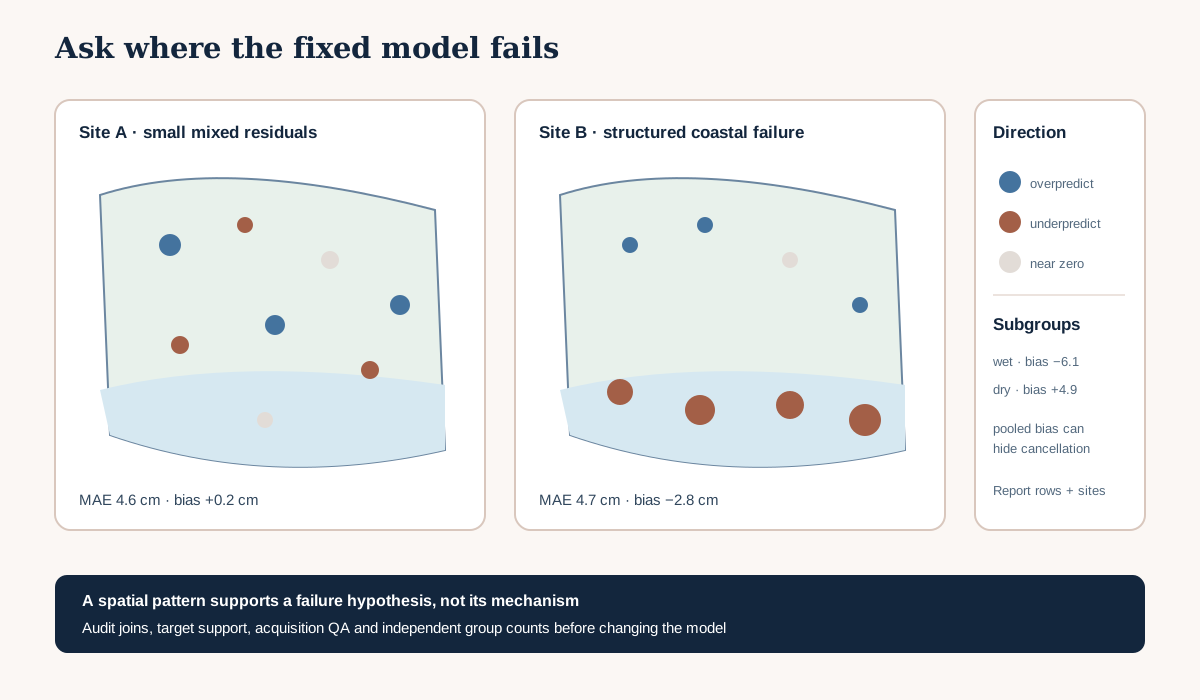
The first map’s residuals are small and mixed. The second contains a spatial band of negative residuals. If only the pooled MAE is shown, the scientific difference disappears. The map needs a symmetric colour scale around zero, accessible symbols and a clear statement of residual sign. Magnitude can be encoded separately from direction.

5. Worked example — summarise residuals by a trusted subgroup

Predict before running

Suppose the overall bias is nearly zero, but wet habitat is consistently underpredicted and dry habitat overpredicted. What will happen when the groups are pooled? Which table column will reveal cancellation most directly?

diagnostic = outer_predictions.merge(
    context_registry,
    on="observation_id",
    how="left",
    validate="one_to_one",
)
if diagnostic["site"].isna().any():
    raise ValueError("Every prediction needs trusted context")

diagnostic["residual"] = (
    diagnostic["prediction"] - diagnostic["observed"]
)
diagnostic["absolute_error"] = diagnostic["residual"].abs()

by_habitat = diagnostic.groupby("habitat_stratum").agg(
    n=("observation_id", "size"),
    sites=("site", "nunique"),
    mae_cm=("absolute_error", "mean"),
    bias_cm=("residual", "mean"),
)
by_habitat

Code walkthrough

1. The join uses a stable identity, not coordinate proximity.
2. how="left" preserves every protected prediction row.
3. validate="one_to_one" blocks duplicated context or predictions.
4. Missing site values signal incomplete context and stop analysis.
5. Residual sign matches Lesson 3.17.
6. Absolute error separates magnitude from direction.
7. Grouping uses a documented context field.
8. n prevents a two-row subgroup from appearing equally supported.
9. Unique sites distinguish rows from independent spatial contexts.
10. MAE measures typical magnitude inside the subgroup.
11. Bias reveals systematic direction and cancellation.
12. The table identifies a pattern; it does not identify its cause.

Diagnostic check

Compare the joined row count and ID set with the original prediction registry. Verify context provenance and meaning. Plot subgroup target distributions; a high-error group may simply contain a more difficult target range. Retain fold and site columns so repeated rows from one site are not mistaken for independent replication.

6. Map regression residuals responsibly

Produce one diagnostic map per outer assessment site or a faceted figure. Use the native prediction-unit support rather than oversized points that imply wider coverage. Recommended views are:

• signed residual with a diverging scale centred at zero;
• absolute error with a sequential scale;
• observed target or predicted value in a companion panel;
• outline of the evaluated site and an explicit “synthetic generalized coordinates” note.

Do not interpolate sparse residual points into a continuous surface unless an interpolation method, support and uncertainty are part of the question. A smooth residual raster can suggest evidence between samples that was never observed.

If using a spatial statistic such as Moran’s I, declare the neighbourhood definition and use it as one diagnostic. The statistic is sensitive to weights, sampling and boundaries. Map the residuals and report the design rather than presenting one p-value as a mechanism.

7. Diagnose important structures

Site

Site-level folds are the first transfer unit. Report metrics, counts, target range and predictor support. A failed site can dominate operational risk even when pooled performance passes.

Habitat or community stratum

Use only documented meanings. Compare target and predictor distributions before attributing error to ecological type. Small or single-site strata cannot establish general habitat performance.

Management

Management may be a predictor, stratifier or unmeasured hypothesis. Its recorded categories may summarize complex histories. Do not interpret association as a management effect.

Environmental gradient

Bin a gradient only with a declared rule, preferably defined before looking at residuals. Continuous residual-versus-gradient plots preserve more information. Investigate edge-of-range failures and non-constant variance.

Acquisition condition

Cloud, haze, solar geometry, phenological mismatch, UAV flight condition or product quality can structure model error. These are candidates for upstream QA, not excuses to remove difficult rows after evaluation.

Spatial region

Compare coastal/inland bands, blocks or geographic zones that match the prediction decision. Avoid repeatedly searching arbitrary partitions until a dramatic difference appears. Exploratory discoveries must be labelled and tested on new evidence.

8. Classification failure geography

Create an error_type field with true positive, false positive, true negative and false negative. Map false negatives prominently when missing rare habitat has high consequence, but also show false-positive review burden. A cluster of false positives near water may indicate spectral confusion, support mismatch or a prevalence difference; it does not prove one feature caused them.

Report class counts by site and subgroup. A group with no reference positives cannot demonstrate sensitivity. If rare habitat occurs at only one site, site and class are confounded; the correct conclusion is insufficient independent representation.

Check your understandingWhat must accompany a subgroup MAE?

Choose one answer

Observation count, independent-site count, target/class support and fold contextOnly the subgroup nameA smooth residual surface

Check answer

9. Predeclared evaluation versus post-hoc discovery

The experiment plan should name high-priority groups before model evaluation when equity, safety or ecological importance requires guarantees. These are confirmatory diagnostics. Additional patterns discovered after viewing residuals are exploratory hypotheses.

For every discovered pattern, record:

• the exact subset and rule that produced it;
• whether it was predeclared;
• observation and independent-site counts;
• effect size with uncertainty or observed spread;
• plausible data-quality and support explanations;
• plausible modelling explanations;
• new data or held-out evidence needed for confirmation;
• whether current deployment must be restricted meanwhile.

Do not run dozens of partitions and publish only the worst one. That is diagnostic selection bias.

10. Data-quality triage before model revision

Large or clustered residuals require a source audit:

1. Is the target record valid and within protocol?
2. Were units and transformations preserved?
3. Do field and predictor dates match the declared temporal support?
4. Is the plot-to-cell reconciliation correct?
5. Did cloud, shadow, saturation, georegistration or NoData affect inputs?
6. Was the feature schema identical at fit and predict time?
7. Is the row environmentally outside training support?
8. Is the error a valid observation of model limitation?

Only documented data errors justify correction or exclusion under a versioned rule. A scientifically inconvenient residual is not a data error.

11. Model clinic — maps that tell more than the evidence

“The red cluster proves salinity causes underprediction”

Salinity was not observed, and coastal distance correlates with several processes. Report a spatial error cluster and a hypothesis requiring salinity measurements.

“Habitat B has twice the MAE”

Habitat B contains three rows from one site and a wider target range. Report counts, site representation and uncertainty; do not generalise.

“Adding coordinates fixed the map”

Random validation improved because coordinates helped identify location. New-site transfer worsened. Evaluate coordinates under the intended spatial fold and justify operational meaning.

“We interpolated residuals for clarity”

Sparse assessment points became a continuous-looking error field without support or uncertainty. Return to observation symbols or design a valid interpolation study.

“Bad-weather rows were removed”

The removal was decided after seeing large errors. Treat it as a new QA procedure and seek fresh assessment.

12. Common mistakes

Joining context many-to-many

Why beginners make it: duplicated keys are not visible. Recognition: row count increases after the join. Fix: validate key uniqueness and expected cardinality. Consequence: errors receive duplicated influence.

Using a non-centred colour scale

Why: automatic scaling maximises contrast. Recognition: zero is not visually neutral. Fix: use symmetric limits or clearly justify asymmetric operational thresholds. Consequence: direction is visually distorted.

Comparing subgroup metrics without target distributions

Why: the table seems sufficient. Recognition: one group contains all extreme targets. Fix: report target and predictor ranges. Consequence: difficulty and group identity are confounded.

Treating pixels as independent sites

Why: there are many rows. Recognition: confidence is driven by dense sampling from one location. Fix: report independent groups and use the Chapter 3 fold unit. Consequence: evidence precision is overstated.

Editing the model during diagnosis

Why: the failure suggests an easy fix. Recognition: outer residuals choose a new feature and the same metrics are reused. Fix: freeze the diagnostic report; preregister a new procedure for new evidence. Consequence: assessment becomes development.

13. Guided practice — build the Model Diagnostic Report

1. Add ## Lesson 3.19 checkpoint to the cumulative notebook.
2. Load regression and classification outer predictions without refitting.
3. Join diagnostic_context.csv by unique observation ID with cardinality validation.
4. Confirm the row set, fold and evidence role were preserved.
5. Calculate signed and absolute regression residuals.
6. Create classification error types at the frozen threshold.
7. Map regression residuals by site with a zero-centred scale.
8. Map false positives and false negatives with distinct shapes and text equivalents.
9. Summarise error by site, habitat, management, gradient band and acquisition condition.
10. Include observations, independent sites and target/class distributions in every summary.
11. Compare patterns across folds rather than only pooled rows.
12. Audit the largest errors against source and QA fields.
13. Classify each finding as predeclared evidence or exploratory hypothesis.
14. Write a confirmation requirement and current deployment consequence for every serious failure.
15. Save structured_failure_summary.csv, maps and the report.

14. Independent challenge — distinguish three explanations for one coastal pattern

An underprediction band appears near the synthetic shore. Develop three competing hypotheses: unrepresented wet vegetation structure, optical/acquisition contamination, and spatial support mismatch. For each, name the additional variable, QA record or sampling design that could discriminate it. State what the current residual pattern supports and what it cannot establish.

Then decide whether the current model may be used in the band, used with a review flag or withheld. The decision must refer to magnitude, representation and consequence, not aesthetic map quality.

15. Scientific interpretation

Residual structure narrows the model’s claim. If errors cluster at a site, subgroup or acquisition condition, the pooled metric does not apply uniformly. The model may still be useful inside better-supported contexts, but the report must expose the difference and define review or withholding rules.

Structured failure is evidence about the predictive system: target, inputs, processing, sampling, model and deployment context together. It is not a direct map of ecological mechanisms. Lesson 3.20 interprets model reliance with the same caution; Lesson 3.21 formalises environmental support before map-wide prediction.

16. Submission

Submit:

• the executed Lesson 3.19 notebook checkpoint;
• structured_failure_summary.csv with counts, fold/site representation and estimability notes;
• spatial_residuals.png and classification error map with accessible descriptions;
• failure_hypotheses.csv separating observation, hypothesis, alternative explanations and required evidence;
• MODEL_DIAGNOSTIC_REPORT.md with supported failures, data-quality audit, deployment consequences and limits;
• a 200–300 word interpretation of the most consequential pattern.

The submission is not acceptable if it hides small groups, smooths sparse residuals into unsupported surfaces, edits the model from outer evidence or claims a causal mechanism from geographic association.

17. Portfolio artifact

Model Diagnostic Report — Chapter 5, Part 3

This report combines performance with the geography and context of failure. It is a professional review artifact: a decision-maker can see which contexts are supported, which require investigation and which must not inherit the pooled metric. Lessons 3.20–3.21 add explanation boundaries and applicability gates.

18. Reflection

1. Which subgroup finding was predeclared and which was discovered?
2. What did the map reveal that pooled MAE did not?
3. Which candidate explanation could be checked using existing QA records?
4. When would adding coordinates harm the intended transfer claim?
5. Which region would you flag before any new model is built?

Check your understandingA new feature is suggested by outer residuals. What is the defensible next step?

Choose one answer

Preregister a revised procedure and evaluate it on fresh protected evidenceAdd it and quote the same outer resultsDelete the failed subgroup

Check answer

19. Core references

• Roberts et al. (2017), cross-validation strategies for structured data
• scikit-learn — model evaluation
• GeoPandas — merging data

Further advanced reading

• Valavi et al. (2019), blockCV spatial and environmental blocking
• Ploton et al. (2020), spatial validation and forest carbon maps

20. Tested software versions

Teaching examples were reviewed for Python 3.12.13, JupyterLab 4 / Notebook 7, NumPy 2.4.2, pandas 2.2.3 and scikit-learn 1.9.0. Mapping assumes the already-tested Module 2 geospatial environment. All supplied coordinates, contexts, labels and errors are deterministic synthetic teaching evidence.