Classification Evaluation and Probability Quality

1. Problem — labels, rankings and probabilities are three different products

Learning outcome

By the end of this lesson, you will be able to evaluate a fixed binary classifier using confusion counts, precision, recall/sensitivity, specificity, F1 and balanced accuracy; distinguish threshold-specific decisions from threshold-free ranking summaries; construct and interpret ROC and precision–recall curves under class imbalance; calculate the Brier score; read a reliability diagram with bin counts; and decide whether a probability estimate is sufficiently calibrated for a bounded rare-habitat screening use.

• Lesson type: Classification and Probability-quality Laboratory
• Estimated time: 230–310 minutes
• Prerequisites: Lesson 3.16 threshold policy and protected outer probabilities; Chapter 3 evidence roles
• Portfolio outputs: classification_metrics_by_fold.csv, probability_quality.csv, classification_diagnostic_figure.png, and CLASSIFICATION_EVALUATION.md

Why this matters

A classifier can rank rare habitat above other meadow units reasonably well while producing badly calibrated probabilities. It can have a high ROC-AUC yet deliver poor precision at the small part of the ranking where a field team can act. It can achieve a desired recall while generating more false-positive visits than the survey budget permits. These are not contradictions. They describe different properties of the score and decision system.

Remote-sensing maps often display model scores as probabilities. That visual convention can invite an unjustified interpretation: a pixel labelled 0.8 appears to mean an 80% chance of habitat. Such a claim requires probability-quality evidence in conditions matching use. Ranking evidence alone is insufficient, and class weighting or prevalence shift can further change calibration.

Core lesson: evaluate the fixed class decision, the ordering of scores and the meaning of probability values separately.

Mental model

fixed classifier → score/probability → ranking evidence
                         ↓
                  calibration evidence
                         ↓
             fixed Chapter 4 threshold → class decision evidence

2. Scientific context — rare-habitat screening with a limited review budget

The Chapter 4 threshold record defined the positive class as rare habitat under a documented reference protocol and selected an action threshold from structured development predictions. Chapter 5 does not move that threshold. It assesses the fixed classifier-plus-threshold procedure on protected outer folds.

The intended use is screening: prioritise mapped units for expert review. The classifier does not certify legal habitat status, replace field verification or estimate a universal habitat prevalence. The supplied outer probabilities are synthetic and deliberately include a site with prevalence and calibration differences.

Preserve the reference label, probability for the declared positive class, fixed predicted label, site, fold and evidence role. If predict_proba returns two columns, verify class order from model.classes_; do not assume the second column has the intended meaning without checking.

3. Concept — decision metrics begin with the confusion matrix

For positive rare habitat, the matrix contains TP, FP, TN and FN. Lesson 3.16 introduced precision, recall and specificity. Add:

$$F1 = 2\frac{precision \times recall}{precision + recall}$$

F1 balances precision and recall through a harmonic mean. It ignores true negatives and does not encode the actual consequence of either error. A high F1 is not automatically a defensible conservation decision.

$$Balanced\ accuracy = \frac{sensitivity + specificity}{2}$$

Balanced accuracy gives equal weight to the reference positive and negative classes. It helps reveal majority-class dominance but still does not describe probability quality, workload or prevalence-specific precision.

In land-cover accuracy terminology, recall for a mapped class is closely related to producer’s accuracy: how much reference class was captured. Precision is closely related to user’s accuracy: how often mapped class members agree with reference. State orientation because matrix conventions differ among software and disciplines.

Check your understandingWhich evidence evaluates the one frozen operational threshold?

Choose one answer

Confusion counts and their derived decision metricsROC-AUC aloneA reliability diagram alone

Check answer

4. Visual explanation — three questions, three evidence views

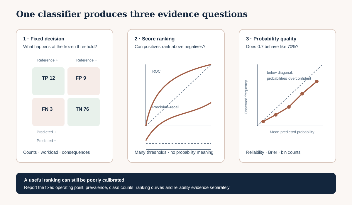
The confusion matrix belongs to one fixed threshold. ROC and precision–recall curves examine many thresholds and therefore describe ranking trade-offs. The reliability panel compares predicted probability with observed frequency in bins and describes probability meaning. Do not use one view to answer all three questions.

5. Worked example — evaluate the fixed threshold and probability quality

Predict before running

Suppose probabilities are consistently too high but preserve the correct ordering. Which may remain strong: ROC-AUC or calibration? Will changing only the threshold repair the meaning of 0.8? Record your answers.

from sklearn.metrics import (
    balanced_accuracy_score, brier_score_loss, confusion_matrix,
    f1_score, precision_score, recall_score, roc_auc_score,
)

y_true = outer_scores["rare_habitat"].to_numpy()
probability = outer_scores["rare_probability"].to_numpy()
predicted = (probability >= frozen_threshold).astype(int)
tn, fp, fn, tp = confusion_matrix(y_true, predicted, labels=[0, 1]).ravel()

metrics = {
    "precision": precision_score(y_true, predicted, zero_division=0),
    "recall": recall_score(y_true, predicted, zero_division=0),
    "specificity": tn / (tn + fp),
    "f1": f1_score(y_true, predicted, zero_division=0),
    "balanced_accuracy": balanced_accuracy_score(y_true, predicted),
    "roc_auc": roc_auc_score(y_true, probability),
    "brier": brier_score_loss(y_true, probability),
}
metrics

Code walkthrough

1. Every function receives protected outer evidence.
2. y_true names the reference positive class explicitly.
3. probability must correspond to that same class.
4. The threshold is frozen from Chapter 4 development evidence.
5. labels=[0, 1] fixes confusion-matrix order.
6. Precision describes the purity of flagged units.
7. Recall describes the captured reference positives.
8. Specificity describes correctly unflagged reference negatives.
9. F1 combines precision and recall but ignores true negatives.
10. Balanced accuracy averages sensitivity and specificity.
11. ROC-AUC uses continuous scores and does not evaluate the one fixed action threshold.
12. Brier loss averages squared differences between probabilities and binary outcomes; lower is better.

Diagnostic check

Report TP, FP, TN and FN beside every rate. Confirm both classes occur before calculating AUC. Preserve the threshold, positive class, prevalence, site counts and evidence role. A fold with no positives cannot support recall or ROC-AUC; do not silently replace undefined evidence with zero.

6. ROC curves — ranking across false-positive rates

A receiver operating characteristic curve plots sensitivity against false-positive rate across thresholds:

$$FPR = \frac{FP}{FP + TN} = 1 - specificity$$

ROC-AUC is the probability that a randomly selected positive receives a higher score than a randomly selected negative, with tie handling defined by the implementation. It measures ranking, not calibration. It can be useful across prevalences because its axes condition separately on each class.

Under strong imbalance, however, a small false-positive rate can still represent many false positives because negatives are abundant. The operationally relevant low-FPR region may occupy a tiny part of the full plot. Never claim ROC-AUC is mathematically invalid under imbalance; explain instead why it may be insufficient for the intended workload and must be paired with class counts and precision–recall evidence.

7. Precision–recall curves — positive retrieval and prevalence

A precision–recall curve plots precision against recall as the threshold changes. It focuses attention on the positive class and the false positives among flagged units. The no-skill precision baseline equals positive prevalence in the evaluated sample. Therefore PR curves and average precision are prevalence-dependent; a value does not transfer unchanged to a population with a different class rate.

For rare-habitat screening, show the fixed operating point on the curve and report the number flagged. If the field team can inspect 40 units, an impressive curve outside that workload region is less relevant. Precision and recall should inform, not replace, the predeclared ecological decision rule.

Check your understandingWhy pair ROC with precision–recall evidence for a rare class?

Choose one answer

A small false-positive rate can still create many false positives, while precision shows positive retrieval at the evaluated prevalenceROC-AUC is undefined whenever classes are imbalancedPrecision–recall curves are independent of prevalence

Check answer

8. Probability calibration — does 0.7 behave like 70%?

A classifier is calibrated when, among comparable predictions near a probability value, the observed event frequency is similar. A reliability diagram groups probabilities into bins, then plots mean predicted probability against the observed positive fraction. The diagonal is perfect empirical reliability.

Bins require care:

• equal-width bins can contain very few observations at probability extremes;
• equal-frequency bins contain similar counts but different probability widths;
• few positives produce step-like observed fractions;
• pooling sites can hide site-specific miscalibration;
• calibration estimated on training predictions is optimistic;
• a post-hoc calibrator must be fitted inside development evidence and assessed on new protected evidence.

Display bin counts and uncertainty or at least the positive count. A smooth diagonal from tiny bins is not strong proof.

Brier score

For binary outcomes:

$$Brier = \frac{1}{n}\sum_{i=1}^{n}(p_i-y_i)^2$$

The Brier score jointly reflects calibration and discrimination; lower is better. It should be compared with a declared reference probability forecast, such as training-fold prevalence, on the same rows. A single Brier value cannot identify whether weakness comes from poor ranking or miscalibration, so retain the reliability diagram and score distributions.

Calibration is model development

Platt/sigmoid or isotonic calibration learns from labels. It belongs inside the Chapter 3 development structure. Do not fit a calibrator on outer assessment probabilities and then report the same outer Brier score as neutral. If Chapter 5 diagnoses miscalibration and proposes a calibrated version, that is a new procedure requiring fresh protected assessment.

9. Fold and subgroup reporting

Calculate decision and probability metrics by outer site where estimable. Always report:

• positives, negatives and prevalence;
• TP, FP, TN and FN at the fixed threshold;
• precision, recall, specificity, F1 and balanced accuracy;
• ROC-AUC and average precision when both classes and sufficient evidence exist;
• Brier score and reliability-bin counts;
• number and proportion flagged;
• score distribution by reference class.

Do not average undefined fold metrics into a seemingly complete table. If a site contains no reference positives, it can contribute specificity, false-positive burden and Brier evidence, but not site-specific recall or ROC-AUC.

10. Model clinic — polished classification claims that collapse under inspection

“ROC-AUC is 0.91, so the habitat map is 91% accurate”

ROC-AUC is a ranking statistic across thresholds, not percentage accuracy at the fixed action. Report the operating confusion matrix and probability quality.

“The score is 0.8, so the patch has an 80% chance of habitat”

The reliability plot shows comparable scores are positive only 55% of the time. Call the output a model score unless calibration evidence supports probability language in the domain.

“F1 selected the objectively best threshold”

F1 encodes a particular balance, ignores true negatives and field capacity, and was evaluated after inspecting protected labels. Restore the Chapter 4 predeclared threshold rule.

“PR-AUC solves class imbalance”

The metric focuses on positive retrieval but depends on prevalence and does not repair limited positive sites, biased sampling or miscalibration.

“The pooled classifier is calibrated”

One common site dominates. Reliability differs at the held-out rare site. Show fold evidence and restrict the claim.

11. Common mistakes

Assuming probability-column order

Why beginners make it: examples use column 1 for the positive class. Recognition: probabilities appear inverted. Fix: inspect classes_ and select by the declared label. Consequence: every metric and threshold is reversed.

Hiding zero denominators

Why: software warnings seem inconvenient. Recognition: recall is reported as zero for a fold containing no positives. Fix: report “not estimable” with counts. Consequence: absence of evidence is misrepresented as poor performance.

Calibrating on assessment data

Why: calibration functions need labels and the outer labels are available. Recognition: the same rows fit and score the calibrator. Fix: calibrate inside structured development; assess once outside it. Consequence: probability quality is optimistic.

Comparing PR-AUC across different prevalences without context

Why: area values look standardized. Recognition: datasets have different positive rates. Fix: report prevalence and the baseline, and prefer matched evaluation sets for model comparisons. Consequence: ranking claims are misleading.

Reporting rates without workload

Why: percentages feel complete. Recognition: no count of flagged units or false positives exists. Fix: link the operating point to review capacity. Consequence: an unusable decision looks successful.

12. Guided practice — build the class and probability evidence record

1. Add ## Lesson 3.18 checkpoint to the cumulative notebook.
2. Load classification_outer_probabilities.csv and verify evidence roles.
3. Name the positive class and verify probability-column meaning.
4. Apply the frozen Chapter 4 threshold without adjustment.
5. Calculate and preserve all four confusion counts.
6. Calculate precision, recall, specificity, F1 and balanced accuracy.
7. Plot ROC and precision–recall curves; mark the fixed operating point.
8. Record ROC-AUC, average precision and evaluation prevalence.
9. Calculate Brier score for the candidate and training-prevalence reference forecast.
10. Build equal-frequency reliability bins with count and positive count.
11. Repeat by outer site only where a metric is estimable.
12. Compare score ranking with probability reliability.
13. Calculate the number of units sent to review at the fixed threshold.
14. State whether probability language is supported or whether “score” is safer.
15. Save the figure, tables and decision report without fitting a calibrator on outer evidence.

13. Independent challenge — a strong ranking with weak probabilities

The fixture includes an intentionally overconfident site. Demonstrate how ROC-AUC can remain useful while the reliability diagram and Brier score reveal poor probability meaning. Then draft a versioned development proposal for calibration. Specify where the calibrator would fit, which groups would validate it, which metric would select it and which independent evidence would assess it.

Do not execute the revision on the current outer targets. The challenge is to design the next experiment, not reuse assessment labels.

14. Scientific interpretation

The fixed classifier may support a bounded prioritisation statement if protected evidence shows useful rare-habitat retrieval at an acceptable review burden. Ranking, threshold behaviour and calibration qualify different parts of that statement. The result does not establish habitat presence, universal prevalence, legal status or causal ecology.

If the score is poorly calibrated, it can still rank candidates but should not be communicated as a literal probability. If performance differs among sites, the pooled metric must be restricted. Lesson 3.19 will investigate whether these differences follow geography, habitat, management or acquisition structure.

15. Submission

Submit:

• the executed Lesson 3.18 notebook checkpoint;
• classification_metrics_by_fold.csv with counts, prevalence and estimability flags;
• probability_quality.csv with Brier comparison and reliability-bin evidence;
• classification_diagnostic_figure.png containing confusion, ROC, PR and reliability views with accessible explanation;
• CLASSIFICATION_EVALUATION.md defining the positive class, threshold, intended action, supported claim and probability-language decision;
• a 200–300 word written answer distinguishing classification, ranking and calibration.

The submission fails review if it changes the threshold from outer evidence, calls ROC-AUC accuracy, omits prevalence or claims unassessed probabilities are calibrated.

16. Portfolio artifact

Classification Evaluation and Probability-quality Package — Chapter 5, Part 2

This artifact records the complete class-decision system rather than one metric. It joins the regression package in the Model Diagnostic and Applicability Package. Lesson 3.19 will ask whether either task has geographically or ecologically structured failure.

17. Reflection

1. Which metric answers the fixed field-review decision most directly?
2. Why can useful ROC-AUC coexist with poor probability calibration?
3. How does prevalence affect precision and the PR baseline?
4. When is a fold-specific metric not estimable?
5. What new evidence would a calibrated model require?

Check your understandingMay outer assessment labels fit a calibrator and also assess its Brier score?

Choose one answer

No; calibration is learned model development and needs fresh protected assessmentYes; calibration never changes predictionsYes, whenever reliability improves

Check answer

18. Core references

• scikit-learn 1.9 — classification metrics
• scikit-learn 1.9 — probability calibration
• scikit-learn — precision–recall

Further advanced reading

• Saito and Rehmsmeier (2015), precision–recall and ROC under imbalance
• Gneiting and Raftery (2007), proper scoring rules
• Sofaer et al. (2019), precision–recall for rare ecological events

19. Tested software versions

Teaching examples were reviewed for Python 3.12.13, JupyterLab 4 / Notebook 7, NumPy 2.4.2, pandas 2.2.3 and scikit-learn 1.9.0. XGBoost 3.3.0 remains the fitted model environment. The supplied probabilities and labels are deterministic synthetic teaching evidence and do not estimate real Baltic habitat prevalence or performance.