Model Interpretation Without Causal Overclaiming

1. Problem — model explanation can become a causal story faster than evidence allows

Learning outcome

By the end of this lesson, you will be able to distinguish global from local model explanations; compare XGBoost gain, held-out permutation importance, partial dependence, individual conditional expectation and SHAP; describe what each method measures and assumes; diagnose instability caused by correlated predictors and unsupported feature combinations; and write predictive interpretations that do not claim ecological mechanism or causal effect.

• Lesson type: Predictive Interpretation and Claim-boundary Laboratory
• Estimated time: 240–320 minutes
• Prerequisites: Lesson 3.15 feature stability; Lessons 3.17–3.19 diagnostic evidence; Chapter 1 prediction-versus-causality contract
• Portfolio outputs: interpretation_method_comparison.csv, interpretation_stability.png, INTERPRETATION_CLAIMS.md, and notebook checkpoint

Why this matters

Tree models can produce convincing explanation graphics. A bar says one index is important. A dependence curve rises. A SHAP plot attributes 4 cm of a prediction to canopy height. These outputs are useful descriptions of a fitted predictive function. They can also tempt the analyst to write that the index controls biomass, that increasing it would cause taller vegetation, or that a local attribution reveals the true ecological mechanism.

That leap is not justified. Predictors can be proxies for site, season, management or acquisition conditions. Correlated variables can exchange apparent importance. Partial-dependence combinations may be rare or impossible. SHAP values depend on the fitted model and background/interventional assumptions. A model trained to predict from observational data does not become a causal experiment because an explanation library was applied.

Core lesson: explain how the fitted model used available information, then stop at the boundary of predictive evidence.

Mental model

fitted predictive function + evaluation data + explanation rule
                              ↓
           global reliance · average response · local attribution
                              ↓
             stability checks · correlation · support checks
                              ↓
           predictive statement ≠ intervention ≠ mechanism

2. Scientific context — explaining a fixed vegetation model after validation

The research group wants to know how the fixed XGBoost vegetation-height model uses EO predictors. The model has already passed or failed the preceding evaluation; interpretation does not rescue weak validation. Use only the frozen feature schema and saved model version.

Candidate features include synthetic UAV canopy-height summaries, Sentinel-2 vegetation indices, moisture-sensitive information, texture and acquisition context. Some are correlated. Their names and units are explicit in the teaching pack. They do not establish real Baltic relationships.

Separate two audiences. A modelling reviewer needs method settings, background data, metric and stability. An ecological collaborator needs plain language: which predictors the model relied on, over which represented ranges, with which caveats, and what cannot be inferred.

3. Concept — five explanation families answer different questions

XGBoost gain importance

Gain aggregates improvement in the training objective attributed to splits using a feature. It is fast and model-internal. It reflects how the fitted trees used features during training, not how much held-out performance depends on them. Features with many candidate split points and correlated alternatives can receive uneven credit. Gain is neither an effect size nor causal importance.

Permutation importance

Held-out permutation importance measures how much a chosen evaluation score degrades when one feature is shuffled. It describes reliance of this model, for this metric, on this evaluation distribution. Correlated features can substitute for each other, making individual importance appear small. Spatially naive shuffling may create impossible combinations; grouped or conditional approaches require careful design.

Partial dependence

Partial dependence estimates the model’s average prediction as one feature is varied while averaging over other observed feature values. It describes the fitted response surface. When features are correlated, varying one independently can create combinations outside the data manifold. Restrict the grid to represented ranges and show data density.

Individual conditional expectation

ICE traces the fitted prediction for each observation while varying one feature. It reveals heterogeneous model responses hidden by the partial-dependence average. The same support and correlation cautions apply. ICE curves are model probes, not subject-specific causal trajectories.

SHAP

SHAP methods allocate a prediction relative to an expected model output among features under a chosen explanation formulation. TreeExplainer can efficiently explain tree ensembles. Global summaries aggregate local attributions; local waterfall plots explain one model output. Results depend on the fitted model, feature dependence assumptions and background data. An attribution is not the amount an ecological process caused the target.

Check your understandingWhat does held-out permutation importance estimate?

Choose one answer

How much this fitted model's chosen score degrades when one feature is disrupted on that evidenceThe feature's causal ecological effectThe sensor's universal physical importance

Check answer

4. Visual explanation — stable predictive statements survive more than one lens

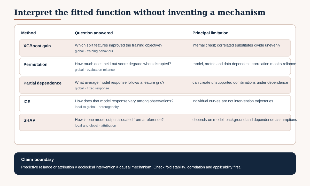
No method is the universal truth. Agreement can strengthen a bounded statement such as “the fitted model relies repeatedly on canopy-height information in represented folds.” Disagreement is also evidence: it may reveal redundancy, interaction, distribution shift or explanation assumptions that require investigation.

5. Worked example — compare gain with protected permutation reliance

Predict before running

Two highly correlated vegetation indices appear in the model. Gain ranks one first and the other low. What might happen to individual permutation importance? Would either result prove that one index is the ecological driver?

import pandas as pd
from sklearn.inspection import permutation_importance

gain = pd.Series(
    fitted_model.feature_importances_, index=feature_order, name="gain"
)
permuted = permutation_importance(
    fitted_model,
    X_outer_assessment[feature_order],
    y_outer_assessment,
    scoring="neg_mean_absolute_error",
    n_repeats=30,
    random_state=42,
)
comparison = pd.DataFrame({
    "gain": gain,
    "permutation_mae_increase": permuted.importances_mean,
    "permutation_spread": permuted.importances_std,
}).sort_values("permutation_mae_increase", ascending=False)
comparison

Code walkthrough

1. The feature order is the saved fit-time schema.
2. feature_importances_ provides XGBoost’s exposed importance values; document the configured importance type.
3. Gain is indexed by actual feature names rather than column positions.
4. Permutation uses protected assessment rows only for diagnosis, not model revision.
5. The scoring rule is the Chapter 4/5 MAE convention.
6. Thirty repeats estimate variation from shuffle order; they do not create new independent sites.
7. A seed makes the diagnostic reproducible.
8. Mean score decrease is expressed as an MAE increase under the negative scorer convention.
9. Spread records shuffle variability.
10. Sorting aids inspection but does not create a causal rank.
11. Repeat this in each outer fold; never let one pooled list hide instability.

Diagnostic check

Confirm the model performs usefully before interpreting it. Record feature correlation, fold, metric, background or assessment dataset, repeats and random seed. Check whether permutation creates implausible combinations. Do not use outer importance to select features and then quote the same outer metrics as independent.

6. Partial dependence and ICE without impossible ecology

Choose one predictor with a clear measurement definition and adequate support. Plot partial dependence only between conservative observed percentiles, then add a rug or histogram showing where data exist. Overlay ICE curves or a representative subset to reveal heterogeneity.

Ask:

• Is the average response monotonic, saturating or threshold-like?
• Do ICE curves share the pattern or cross strongly?
• Which feature values have sparse support?
• Is the predictor strongly correlated with another variable?
• Does the pattern remain across outer-fold models?
• Could acquisition or site identity act as a proxy?

Write “the model’s predicted height increases over the represented NDVI range while other recorded features are averaged over,” not “raising NDVI increases vegetation height.” NDVI is derived from reflectance and not an intervention.

Scikit-learn’s documentation notes that partial dependence and ICE assume the target feature is independent of the complement for interpretable averaging. When that assumption is implausible, narrow the claim, use conditional analysis where justified, or refrain from interpreting the curve.

7. SHAP as local and global model attribution

For a tree ensemble, define a background dataset representing the development distribution and document it. Explain a small, protected diagnostic sample if computation is constrained. Verify the explainer’s output corresponds to the intended model output—raw margin or probability differs for classification.

Use:

• a global distribution summary to show attribution spread;
• one local waterfall for a typical supported case;
• one local waterfall for a high-error or low-applicability case;
• fold-level summaries to examine stability;
• feature-value and attribution plots with density/support context.

Local SHAP values explain how the fitted model moved from its reference output to one prediction under the chosen method. They do not say how the true ecosystem would change if a feature were manipulated. A local explanation outside applicability can faithfully explain an unreliable extrapolation; explanation quality is not prediction validity.

Check your understandingWhat does a local SHAP explanation describe?

Choose one answer

An allocation of this model output relative to a reference under the explainer assumptionsThe intervention effect of changing a featureThe probability that the prediction is correct

Check answer

8. Compare conclusions, not only graphics

Build a method-comparison table with rows for candidate statements and columns for gain, held-out permutation, partial dependence/ICE, SHAP, fold stability, correlation/support caution and allowable wording.

Examples:

• “Canopy-height summary is repeatedly used by the fitted model.”
• “NDVI and red-edge index form a redundant predictive group.”
• “The model response to moisture information differs among represented observations.”
• “One acquisition-condition variable receives high local attribution at the failed site.”

Classify each as stable, conditional, contradictory or unsupported. A stable statement requires agreement across relevant folds and adequate predictor support; it still remains predictive.

9. Correlated predictors and explanation instability

Correlation can distribute credit unpredictably:

• tree splits may choose one of several substitutes;
• gain can concentrate on the chosen member;
• individual permutation can underestimate each substitute;
• partial dependence can traverse implausible combinations;
• SHAP allocations depend on feature-dependence treatment and background data.

Respond by grouping related predictors scientifically, comparing full and reduced schemas from Lesson 3.15, reporting correlation, and checking fold stability. Do not sum SHAP values for an arbitrary group and call it a causal process unless the grouping and explanation semantics are defensible.

10. Claim ladder for interpretation

Move only as high as evidence allows:

1. Model output: “This observation received a prediction of 31 cm.”
2. Model attribution: “Relative to the chosen background, canopy-height information increased this fitted prediction.”
3. Predictive reliance: “Disrupting canopy height reduced held-out performance across represented folds.”
4. Association hypothesis: “The pattern is consistent with canopy structure carrying predictive information.”
5. Mechanism or causal effect: requires an appropriate causal design, assumptions and evidence not supplied by this predictive workflow.

The first four levels still require context. Do not cross to level five with feature-importance language.

11. Model clinic — attractive explanations that exceed the model

“SHAP proves wetness reduces vegetation height by 4 cm”

The value is a local model attribution relative to a background, not an intervention effect. Rewrite it at level two and state applicability.

“Gain and permutation disagree, so one implementation is wrong”

They answer different questions and predictors are correlated. Investigate substitution and fold stability.

“The partial-dependence curve is the ecological response curve”

Sparse high values and correlation create unsupported combinations. Show density and call it a model-response diagnostic.

“The best explanation comes from the best-looking fold”

Selecting one fold hides instability. Preserve every fold and the disagreement.

“Interpretability compensates for weak validation”

A transparent explanation of an invalid or unsupported prediction remains invalid or unsupported. Evaluation and applicability come first.

12. Common mistakes

Interpreting before checking predictive skill

Why beginners make it: explanation plots are compelling. Recognition: no baseline or outer metrics appear. Fix: place the evaluation summary before interpretation. Consequence: noise receives a scientific story.

Using training data for every interpretation

Why: it is readily available. Recognition: permutation reliance describes fitted rows only. Fix: use protected diagnostic evidence and label its role. Consequence: reliance appears optimistic.

Omitting background data from SHAP records

Why: library defaults seem technical. Recognition: attributions cannot be reproduced or interpreted. Fix: save sampling rule, version and explainer configuration. Consequence: reference output and dependence assumptions are hidden.

Treating negative importance as harmful causation

Why: the sign feels causal. Recognition: a feature’s permutation result is below zero in one fold and called ecologically damaging. Fix: interpret as sampling/noise/model instability. Consequence: a random diagnostic becomes mechanism.

Explaining outside the training support

Why: the model returns values everywhere. Recognition: an extrapolated pixel receives a confident waterfall narrative. Fix: attach Lesson 3.21 applicability first. Consequence: an unreliable prediction gains false authority.

13. Guided practice — prepare the interpretation stability record

1. Add ## Lesson 3.20 checkpoint to the cumulative notebook.
2. Restate the predictive—not causal—claim.
3. Load the fixed model, feature order and protected fold predictions.
4. Verify outer performance and note any failed sites from Lesson 3.19.
5. Export XGBoost gain with the configured importance type.
6. Compute permutation importance on each outer fold using the primary metric.
7. Add feature correlation and measurement-role groups.
8. Select two supported predictors for partial dependence and ICE.
9. Restrict grids to represented ranges and display density.
10. Generate SHAP summaries for a documented background and output scale.
11. Compare a typical supported case, a high-error case and a low-applicability candidate.
12. Summarise method agreement and fold stability.
13. Rewrite every interpretation through the claim ladder.
14. Record statements that remain contradictory or unsupported.
15. Save tables, figures, settings and the claim-boundary document.

14. Independent challenge — explain a disagreement among methods

Gain ranks sentinel2_ndvi first, permutation distributes low importance across NDVI and a red-edge index, and SHAP alternates their attribution among folds. Use correlation, feature grouping and fold evidence to explain why this is plausible. Draft one defensible predictive statement and two statements the evidence cannot support.

Then propose an additional validation experiment for a reduced schema. Do not use the current outer results to revise and re-score on the same evidence.

15. Scientific interpretation

Interpretation methods reveal the internal and predictive behaviour of a fixed model under specific data and assumptions. Stable agreement can identify information the model repeatedly uses. Disagreement can reveal redundancy, heterogeneity or fragile reliance. Neither outcome establishes an ecological intervention or causal mechanism.

The strongest scientific report is often less dramatic than the plot: it names the fitted function, evidence, range, metric and limitation. Lesson 3.21 will decide where any explanation accompanies a supported prediction and where the map must be flagged or withheld.

16. Submission

Submit:

• the executed Lesson 3.20 notebook checkpoint;
• interpretation_method_comparison.csv with method question, evidence, settings, fold result and limitation;
• interpretation_stability.png with accessible description and predictor-support context;
• INTERPRETATION_CLAIMS.md containing the claim ladder, supported statements, prohibited causal rewrites and explanation settings;
• one documented local explanation for a supported case and one low-support warning case;
• a 200–300 word response explaining why SHAP is not an ecological mechanism.

The submission fails if it calls feature importance causal, omits correlation/background assumptions, selects predictors from outer explanations and reuses the same performance evidence, or interprets unsupported regions without warning.

17. Portfolio artifact

Interpretation Stability Report — Chapter 5, Part 4

The artifact compares explanation lenses rather than selecting the most persuasive graphic. It connects the diagnostic report to an auditable claim boundary. Lesson 3.21 completes the chapter by mapping where training evidence supports use.

18. Reflection

1. Which method describes internal split gain, and which tests held-out score reliance?
2. Why can partial dependence display unrealistic feature combinations?
3. What does a SHAP value reference?
4. Which predictive statement remained stable across folds?
5. What evidence would be needed for a causal claim?

Check your understandingWhich statement stays inside the predictive claim boundary?

Choose one answer

The fitted model repeatedly relied on canopy-height information across represented foldsIncreasing canopy height will cause the target to riseSHAP proves the ecological mechanism

Check answer

19. Core references

• scikit-learn 1.9 — permutation feature importance
• scikit-learn 1.9 — partial dependence and ICE
• SHAP — TreeExplainer

Further advanced reading

• Molnar, Interpretable Machine Learning
• Apley and Zhu (2020), accumulated local effects
• Shmueli (2010), To Explain or to Predict?

20. Tested software versions

Teaching examples were reviewed for Python 3.12.13, JupyterLab 4 / Notebook 7, NumPy 2.4.2, pandas 2.2.3, scikit-learn 1.9.0 and XGBoost 3.3.0. SHAP is introduced through its current TreeExplainer documentation; learners must record the installed SHAP version and explainer settings because outputs can depend on version and configuration. All data are synthetic.

Interpretation boundary

“High predicted CCI means <i>Juncus gerardi</i> is present” is unsupported unless a separate species-classification model has been trained and validated for that claim. A trait surface is a model output for the specified response, not a botanical inventory. Follow Juncus through the pipeline.