Regression Evaluation

1. Problem — one regression score cannot describe a model’s scientific behaviour

Learning outcome

By the end of this lesson, you will be able to calculate and interpret MAE, RMSE, bias and R² from protected out-of-fold predictions; explain each metric’s units, sensitivity and blind spots; compare the fixed candidate with its baseline on identical observations; diagnose magnitude-dependent error with observed-versus-predicted, residual-versus-fitted and residual-distribution plots; and report fold variability without turning a pooled average into a universal performance claim.

• Lesson type: Regression Evidence and Diagnostic Laboratory
• Estimated time: 220–300 minutes
• Prerequisites: Lessons 3.5 and 3.8; Chapter 3 structured validation; Chapter 4 fixed model-selection procedure
• Portfolio outputs: regression_metrics_by_fold.csv, regression_diagnostic_figure.png, REGRESSION_EVALUATION.md, and notebook checkpoint

Why this matters

A remote-sensing regression rarely fails in only one way. A model can have a respectable R² while systematically underpredicting the tallest vegetation. It can have low mean absolute error because most plots are ordinary while making a few ecologically consequential errors at unusual wet or highly productive sites. It can have zero average bias because positive and negative errors cancel even though both are large. A single pooled metric can also conceal that transfer works at three sites and collapses at a fourth.

Professional evaluation therefore asks a set of linked questions. How large is a typical absolute error? How strongly do large errors influence the result? Is there a systematic direction? How much variation relative to the assessment observations is represented? Does performance vary across the exact sites, blocks or periods that define the claim? What structure remains in the residuals?

Core lesson: a metric is a measurement of one property of prediction error, not a verdict on the model.

Mental model

fixed procedure + protected fold → observed and predicted pairs
                                      ↓
              magnitude · direction · relative variation
                                      ↓
                 plots · fold spread · failure questions
                                      ↓
                       bounded regression claim

2. Scientific context — evaluating vegetation-height transfer

Continue with the synthetic coastal-meadow modelling table and the fixed Chapter 4 procedure. The prediction target is vegetation height in centimetres under the declared field protocol. The intended claim is transfer to represented coastal-meadow sites during the stated growing-season conditions. The final test remains sealed.

Use only outer-fold predictions produced without fitting or selecting on their own target values. Each row must preserve observation_id, site, spatial block, date, observed target, prediction, baseline prediction, outer fold and evidence role. If these fields were discarded, reconstruct them from the saved prediction registry—not by refitting on all data.

The fixture in this chapter is synthetic. Its centimetre values are designed to expose diagnostic patterns. They are not published Baltic coastal-meadow measurements and cannot establish real model performance.

3. Concept — four metrics answer four different questions

Let the residual be:

$$e_i = \hat{y}_i - y_i$$

A positive residual means overprediction under this declared sign convention. State the convention in every report.

Mean absolute error

$$MAE = \frac{1}{n}\sum_{i=1}^{n}|e_i|$$

MAE has the target’s unit: centimetres here. It answers, approximately, “how far are predictions from observations on average, ignoring direction?” Every absolute error contributes linearly. MAE is readable and less dominated by a few large errors than RMSE, but it can hide whether errors are systematic, whether tall vegetation performs worse and whether one site fails.

Root mean squared error

$$RMSE = \sqrt{\frac{1}{n}\sum_{i=1}^{n}e_i^2}$$

RMSE also has the target’s unit. Squaring makes large residuals disproportionately influential. A much larger RMSE than MAE signals a heavy upper tail of errors, though it does not identify their location or cause. RMSE is not automatically “more scientific”; its emphasis is appropriate only when large errors deserve extra influence.

Bias

$$Bias = \frac{1}{n}\sum_{i=1}^{n}e_i$$

With prediction minus observation, positive bias means average overprediction and negative bias means average underprediction. Bias can be near zero through cancellation. Always pair it with magnitude metrics and a residual distribution.

Coefficient of determination

$$R^2 = 1 - \frac{\sum_i(y_i-\hat{y}_i)^2}{\sum_i(y_i-\bar{y})^2}$$

R² compares squared error with a mean-reference model on the same assessment observations. One indicates exact predictions, zero indicates squared error equal to predicting the assessment mean, and negative values are possible when predictions are worse. R² is unitless and depends on target variation in the evaluated sample. A narrow target range can produce low R² alongside a modest MAE; a broad range can produce high R² despite operationally large errors. It is not the proportion of every individual observation “explained,” and it does not prove causality.

Check your understandingWhich statement correctly distinguishes MAE and RMSE?

Choose one answer

Both use the target unit, but RMSE gives large residuals greater influenceMAE is unitless while RMSE has the target unitRMSE always gives the scientifically correct model choice

Check answer

4. Visual explanation — read the metric panel and residual plots together

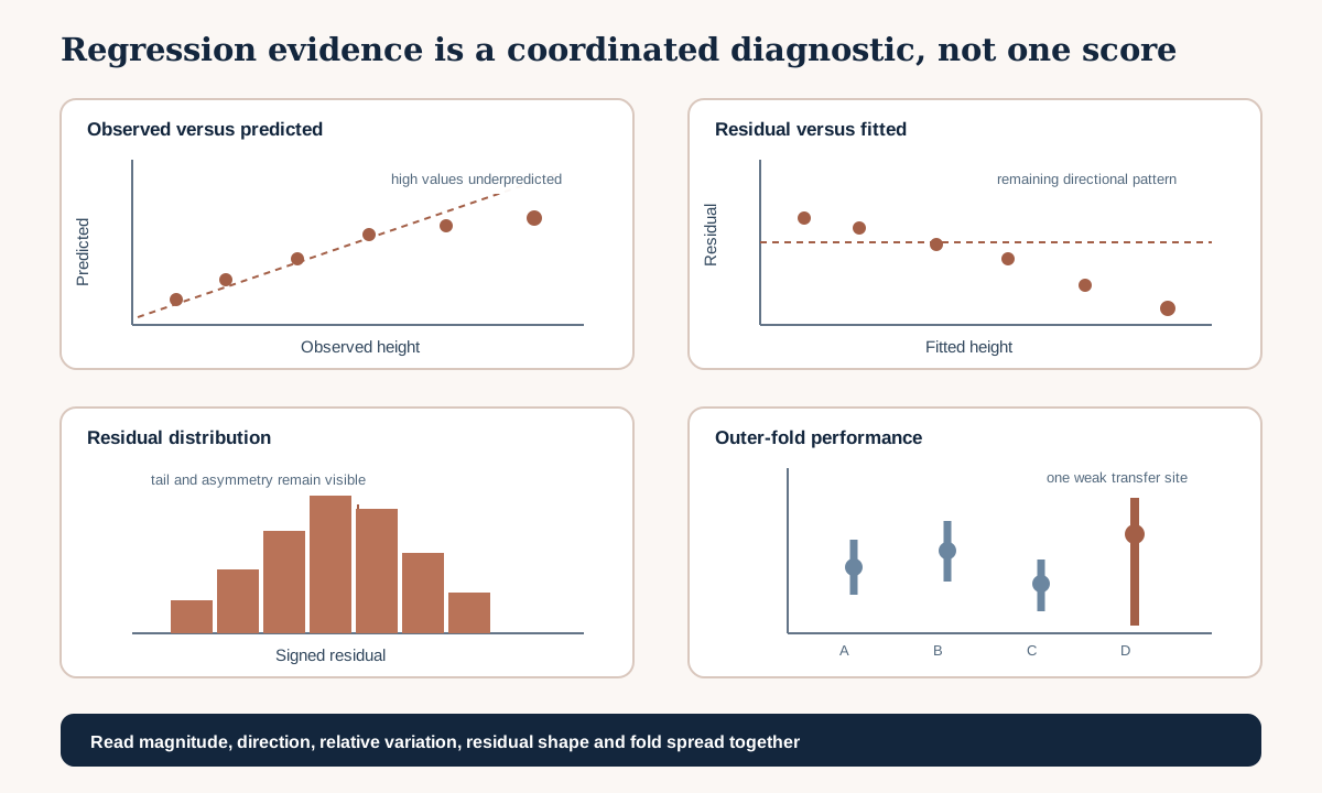
The 1:1 line is a reference, not a fitted trend. Compression toward the mean appears when low observations are overpredicted and high observations are underpredicted. A residual-versus-fitted curve exposes changing bias or variance. The residual distribution shows asymmetry and extreme errors. Fold-level points and ranges show whether a pooled result represents every transfer context.

5. Worked example — calculate the metric set once from saved predictions

Predict before running

Imagine two large underpredictions occur among otherwise small errors. Which will increase more, MAE or RMSE? What sign will bias have? Could R² remain positive? Write your prediction before executing.

from sklearn.metrics import (
    mean_absolute_error, r2_score, root_mean_squared_error
)

evaluation = outer_predictions.copy()
evaluation["residual"] = evaluation["prediction"] - evaluation["observed"]

summary = {
    "n": len(evaluation),
    "mae_cm": mean_absolute_error(
        evaluation["observed"], evaluation["prediction"]
    ),
    "rmse_cm": root_mean_squared_error(
        evaluation["observed"], evaluation["prediction"]
    ),
    "bias_cm": evaluation["residual"].mean(),
    "r_squared": r2_score(
        evaluation["observed"], evaluation["prediction"]
    ),
}
summary

Code walkthrough

1. The imports use scikit-learn’s current named regression metrics.
2. .copy() protects the preserved outer-prediction table from accidental mutation.
3. The residual sign is declared as prediction minus observation.
4. n reports how many rows contribute; a metric without sample size is incomplete.
5. MAE summarises absolute magnitude in centimetres.
6. root_mean_squared_error returns the same unit while emphasising large deviations.
7. Mean residual estimates directional bias under the stated convention.
8. R² compares squared error with the assessment target’s mean reference.
9. Every metric uses exactly the same rows and fixed predictions.
10. The result is a starting summary, not the end of evaluation.

Diagnostic check

Before interpreting the dictionary, assert unique observation IDs, finite paired values, a valid evidence role, and identical rows for model and baseline. Count independent sites and groups. Check that missing observations were excluded by a predeclared rule rather than removed after their errors looked inconvenient.

Check your understandingA held-out site has negative R². What does that mean?

Choose one answer

The fixed predictions have greater squared error than predicting that site's assessment meanThe software failed to calculate a legal valueThe model has negative causal influence

Check answer

6. Compare the candidate with its baseline fairly

Compute the complete metric set for the fixed candidate and the frozen Chapter 2 baseline on identical outer rows. Include absolute skill for the primary metric:

$$MAE\ skill = MAE_{baseline} - MAE_{model}$$

Positive skill means lower model MAE. A percentage improvement can be added only when the baseline denominator is meaningful and non-zero; always retain values in centimetres. If the model improves pooled MAE by 1.2 cm but loses to the baseline at two sites, report both facts.

Never compare the model’s spatial-CV error with a baseline measured on a random split. The evidence design is part of both procedures. Refit each baseline using only the current training fold, then predict its assessment fold.

7. Build the diagnostic figure

Create four coordinated panels from the row-level outer predictions.

Observed versus predicted

Use equal axis scales and draw a 1:1 reference. Encode outer site or fold accessibly with colour plus marker shape. Do not fit a trend line and call it calibration without specifying what it estimates. Inspect range compression, isolated points and site clusters.

Residual versus fitted

Plot prediction on the x-axis and prediction-minus-observation residual on the y-axis. Draw a zero line. Add a restrained smoother only as a diagnostic guide and label it as descriptive. A downward structure may indicate underprediction at high fitted values; a funnel may indicate non-constant error spread.

Residual distribution

Show a histogram or empirical distribution with a zero reference and the mean residual. Do not let a symmetric-looking density replace subgroup checks. Report selected quantiles, including median absolute error and the 90th percentile of absolute error when operationally useful.

Fold performance

Show MAE, RMSE, bias and R² by outer fold with observation and independent-group counts. Because only a few sites may exist, do not present the standard deviation as though folds were random independent draws from every possible Baltic meadow. Call it observed fold spread.

8. What each metric can hide

MAE can hide rare large failures

Many modest errors can dominate the count while two very large errors matter for conservation or field planning. Compare MAE with RMSE, upper absolute-error quantiles and the affected observations.

RMSE can be dominated by a few points

Investigate whether large residuals reflect data errors, unusual but valid conditions, support mismatch or unsupported predictor combinations. Never delete them simply to improve RMSE. Correct only documented errors; valid extremes are evidence about model behaviour.

Bias can cancel

Calculate site, habitat and target-range bias. Positive errors in short vegetation may cancel negative errors in tall vegetation. Pooled zero bias is compatible with a distorted map.

R² changes with the evaluated target distribution

Do not compare R² values across datasets with very different target ranges as though they were directly equivalent. A negative fold R² is not a software failure; it states that the fixed predictions had greater squared error than that fold’s mean reference.

9. Fold summaries and uncertainty in performance

Keep one row per outer fold with metrics, counts, target range and assessment context. Summarise median, minimum and maximum or an explicitly described interval. With only four sites, a polished confidence interval can suggest more independent evidence than exists. The honest report names each site and shows all fold values.

Pooled metrics weight folds by row count. A large site can dominate. An unweighted mean across site metrics answers a different question: the mean of site-specific estimates. Report both only if both correspond to useful claims, and explain their weighting.

Chapter 6 will address prediction uncertainty. Variation of performance across folds is evidence about procedure stability; it is not a prediction interval for an individual pixel.

Check your understandingWhy report fold metrics before a pooled result?

Choose one answer

A pooled average can hide a failed transfer site and weighting by row countEvery fold is an independent estimate of global truthPooling is mathematically prohibited

Check answer

10. Model clinic — plausible summaries that fail review

“R² is 0.78, therefore the model explains 78% of biomass ecology”

R² is turned into a causal statement and the target’s supplied metadata may not even document units. State its mathematical reference, predictive evidence and claim boundary.

“RMSE is more conservative, so the other metrics are unnecessary”

The model has modest RMSE but consistent negative bias in tall vegetation. One metric cannot reveal every failure.

“Average bias is almost zero”

Short vegetation is overpredicted by 6 cm and tall vegetation underpredicted by 7 cm. Stratify by a predeclared target range and inspect residual structure.

“The pooled result represents every site”

Seventy percent of observations come from one easy site. Preserve fold metrics and counts; qualify the domain.

“The extreme plot was removed because it looked wrong”

No source evidence shows an error. Restore it. Investigate data provenance, support and applicability; do not edit evidence from model discomfort.

11. Common mistakes

Reversing the residual sign

Why beginners make it: both definitions appear in practice. Recognition: text says underprediction while the plot’s sign implies overprediction. Fix: write the equation in the notebook and axis label. Consequence: directional conclusions are reversed.

Mixing rows among metrics

Why: each function silently drops or receives different data. Recognition: sample sizes differ. Fix: construct one validated evaluation frame before calculation. Consequence: metrics cannot be compared.

Reporting excessive decimal precision

Why: software returns many digits. Recognition: centimetre error is reported to six decimals despite limited field precision. Fix: preserve calculation precision but display resolution appropriate to the target protocol. Consequence: measurement certainty is overstated.

Pooling before checking folds

Why: one row is easier to communicate. Recognition: no site-specific evidence exists. Fix: calculate fold results first, then a labelled aggregate. Consequence: structured failure disappears.

Treating residual plots as causal diagnosis

Why: a pattern looks mechanistic. Recognition: a curve is attributed directly to grazing or moisture without independent evidence. Fix: state candidate hypotheses and required validation. Consequence: predictive error becomes an unsupported ecological explanation.

12. Guided practice — construct the regression evidence package

1. Add ## Lesson 3.17 checkpoint to the cumulative notebook.
2. Load regression_outer_predictions.csv from the Chapter 5 pack.
3. Validate unique IDs, evidence role, fold, site and finite observed/predicted pairs.
4. Declare the residual sign in prose and code.
5. Calculate candidate and baseline MAE, RMSE, bias and R² on identical rows.
6. Save a pooled table with observation and independent-site counts.
7. Group by outer fold and calculate the same metrics without discarding negative R².
8. Record target minimum, maximum and range per fold.
9. Build the four-panel diagnostic figure with accessible labels and 1:1/zero references.
10. Identify the largest absolute residuals and audit their provenance without automatically excluding them.
11. Write one supported statement for each metric and one property it cannot establish.
12. Compare model and baseline on pooled and site-specific evidence.
13. State whether the model is useful for the declared claim and where evidence is weak.
14. Save stable filenames and leave the final test sealed.

13. Independent challenge — evaluate a model that compresses extremes

The fixture contains a site where tall observations are systematically underpredicted. Without altering the model, quantify the pattern using a predeclared high-target group, the residual plot and site metrics. Compare two possible responses: changing the model now, or recording the failure and carrying it into Chapter 5 diagnosis. Explain which evidence would be required to evaluate a revised procedure honestly.

Your answer must distinguish a data-quality error, a valid but underrepresented condition, and a domain-of-applicability problem. Do not claim one cause from the residual pattern alone.

14. Scientific interpretation

The metric package describes how the fixed procedure predicted held-out synthetic observations under the Chapter 3 design. Lower MAE and RMSE than the baseline support predictive skill for those represented transfers. Bias and residual structure qualify that claim. Fold spread shows the result is not identical across sites.

None of these diagnostics proves why vegetation varies, whether one predictor causes height, or whether performance transfers beyond represented environmental and acquisition conditions. Chapter 3 defines where the predictions were held out; this chapter measures how they failed. Lessons 3.19 and 3.21 will locate structured failure and environmental support.

15. Submission

Submit:

• the executed Lesson 3.17 notebook checkpoint;
• regression_metrics_by_fold.csv containing model and baseline results, counts and target ranges;
• regression_diagnostic_figure.png with descriptive alt text;
• REGRESSION_EVALUATION.md stating the metric definitions, residual sign, supported claim, fold variation, failure pattern and limitations;
• a screenshot showing the four-panel diagnostic figure;
• a 200–300 word written decision on whether the fixed candidate improves usefully over the baseline.

The package is incomplete if it reports only R², omits the baseline, hides fold failures, or changes the model after opening protected predictions.

16. Portfolio artifact

Regression Evaluation Package — Chapter 5, Part 1

This artifact converts preserved outer predictions into a reviewable performance claim. It becomes the quantitative entry to the Model Diagnostic and Applicability Package. Lesson 3.18 adds class decisions, ranking and probability quality; neither lesson may reopen model selection.

17. Reflection

1. Which metric is most directly interpretable in the target unit?
2. What does a large gap between RMSE and MAE prompt you to inspect?
3. How can pooled bias be zero while ecological subgroups remain biased?
4. Why can two datasets produce different R² values for similarly sized errors?
5. Which sentence in your report most clearly limits the transfer claim?

18. Core references

• scikit-learn 1.9 — regression metrics and scoring
• scikit-learn — R² score
• scikit-learn — root mean squared error

Further advanced reading

• Gneiting (2011), Making and Evaluating Point Forecasts
• Roberts et al. (2017), cross-validation strategies for structured data

19. Tested software versions

Teaching examples were reviewed for Python 3.12.13, JupyterLab 4 / Notebook 7, NumPy 2.4.2, pandas 2.2.3 and scikit-learn 1.9.0. XGBoost 3.3.0 remains the fixed candidate environment. The supplied evaluation rows are deterministic synthetic teaching evidence, not measured Baltic coastal-meadow observations.