Imbalanced Classification and Decision Thresholds

1. Problem — a probability model does not decide which meadow patches require action

Learning outcome

By the end of this lesson, you will be able to explain class imbalance and majority dominance; name the positive class explicitly; calculate confusion counts, precision, recall/sensitivity and specificity; distinguish probability estimation from threshold-based action; evaluate class weighting and sampling without leaking assessment; select a rare-habitat decision threshold from a predeclared ecological objective inside structured development evidence; and assess the fixed model-plus-threshold procedure on protected outer folds.

• Lesson type: Rare-habitat Decision Threshold Laboratory
• Estimated time: 220–300 minutes
• Prerequisites: Chapter 3 nested validation and Lessons 3.13–3.15; familiarity with tables, Boolean comparisons and model predictions
• Portfolio outputs: threshold_metrics.csv, RARE_HABITAT_DECISION.md, class-weight comparison, outer confusion records, and the Chapter 4 handover

Why this matters

Rare ecological classes create a deceptive success condition. If only 5 of 100 mapped units contain the habitat of interest, a classifier that predicts “absent” everywhere achieves 95% accuracy. It finds none of the habitat. For survey prioritisation or conservation screening, that behaviour may be scientifically useless.

A classifier commonly produces scores or estimated probabilities. A second rule converts them into labels. The familiar 0.5 probability threshold is a software default, not an ecological law. Lowering it usually identifies more true habitat but also sends more non-habitat units to review. Raising it usually reduces false alarms while missing more true habitat. The defensible choice depends on consequences, field capacity and the reliability of the scores.

Threshold selection is model selection. It belongs inside development evidence. Choosing a threshold from an outer assessment site or final test contaminates that evidence just as surely as choosing max_depth from it.

Core lesson: estimate first, decide second, and evaluate the complete decision rule on evidence that did not choose it.

Mental model

predictors → fitted classifier → score or estimated probability
                                      ↓
                     threshold chosen from development evidence
                                      ↓
                 rare-habitat / other decision labels
                                      ↓
             confusion counts + ecological consequences

outer assessment evaluates classifier + threshold together

2. Scientific context — rare coastal-meadow habitat as a screening decision

Imagine the project is extended from continuous vegetation prediction to screening mapped units for a rare habitat condition. Field observations define presence or absence under a documented protocol. EO predictors describe spectral, moisture, structural and contextual properties at the declared mapping unit.

The operational decision is not “prove habitat from imagery.” It is “prioritise units for expert review under a bounded screening protocol.” A false negative can omit a true patch from follow-up. A false positive consumes field or interpretation capacity. Neither consequence is universally more costly; stakeholders must declare the use.

The lesson fixture contains synthetic labels and synthetic model probabilities. It is deliberately imbalanced and is not evidence of real habitat distribution or classifier performance. In a real application, label quality, prevalence, spatial sampling, probability calibration and survey detectability all require separate review.

3. Concept — define the positive class before calculating anything

For this lesson:

• positive (1): rare habitat is present according to the reference protocol;
• negative (0): rare habitat is absent according to that protocol.

The confusion matrix contains:

• true positive (TP): habitat present and predicted positive;
• false positive (FP): habitat absent but predicted positive;
• true negative (TN): habitat absent and predicted negative;
• false negative (FN): habitat present but predicted negative.

From those counts:

$$\text{precision} = \frac{TP}{TP + FP}$$

Precision asks: among units flagged as rare habitat, what fraction are reference positives?

$$\text{recall or sensitivity} = \frac{TP}{TP + FN}$$

Recall asks: among reference-positive units, what fraction were found?

$$\text{specificity} = \frac{TN}{TN + FP}$$

Specificity asks: among reference-negative units, what fraction were correctly left unflagged?

These quantities answer different questions. Always state the positive class, denominator and evidence role. With very few positive groups, percentages can look precise while representing only a handful of observations. Report counts alongside rates.

Why accuracy can fail

Accuracy divides all correct decisions by all observations. Under severe imbalance, true negatives dominate. It can remain high while recall is zero. Balanced accuracy gives sensitivity and specificity equal influence, but even that does not encode the real consequence or field-review budget. No single metric replaces decision design.

Check your understandingWhat changes when a fitted classifier's decision threshold changes?

Choose one answer

The conversion from scores or probabilities to class actionsThe original field labelsThe sensor's spectral response

Check answer

4. Visual explanation — one score distribution, several possible decisions

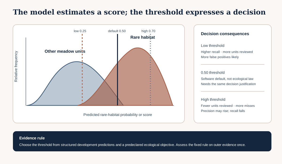
The model scores do not change when the threshold moves. The label decision changes. At a low threshold, most positive units are found but many negative units are flagged. At a high threshold, the flagged set is smaller and may be more precise, but true habitat can be missed.

The overlap between distributions is the difficult region. Thresholding cannot remove that uncertainty. It only expresses one decision trade-off. Chapter 5 will deepen probability quality and classification evaluation; this lesson focuses on selecting the action rule without contaminating evidence.

5. Class imbalance changes fitting and evaluation

Majority dominance

An unweighted training objective can reduce average loss mainly by fitting the abundant negative class. This does not mean the algorithm ignores positives completely, but rare examples contribute less total influence. Site imbalance can make the problem worse: many positive pixels in one site are not equivalent to many independent positive sites.

Class weighting

Class weights increase the contribution of selected observations to the fitting objective. Scikit-learn can compute a balanced heuristic inversely proportional to class frequency. XGBoost exposes scale_pos_weight, often initially considered in relation to negative and positive counts. These are starting points, not automatic ecological costs.

Weighting changes the fitted score function. It can improve minority recall, worsen precision, alter probability calibration and interact with regularisation. Compare it inside the same structured development design.

Sampling approaches

Undersampling removes some majority observations; oversampling repeats or synthesises minority examples. Any target-informed sampling must occur inside training partitions only. Performing it before splitting can place copies or derivatives of one positive source unit across training and validation. Spatial groups and source IDs must remain attached.

Sampling can help computation or fit, but it cannot create new independent habitats or sites. Synthetic minority samples are not new field observations.

Thresholding

Threshold selection leaves fitted scores unchanged and changes the action rule. It is often useful after a candidate classifier has been fitted, but the threshold must be tuned on new development evidence—not on the same rows that trained the estimator and not on protected assessment.

6. Worked example — inspect four thresholds on inner validation

Predict before running

Suppose rare_probability contains scores for a structured inner-validation set. Which metric will usually rise when the threshold is lowered: recall or specificity? Could precision move non-monotonically in a small sample? If 0.35 meets a predeclared minimum recall, may you check the outer site and move it to 0.30?

from sklearn.metrics import confusion_matrix

rows = []
for threshold in [0.20, 0.35, 0.50, 0.65]:
    predicted = (rare_probability >= threshold).astype(int)
    tn, fp, fn, tp = confusion_matrix(
        y_inner_validation, predicted, labels=[0, 1]
    ).ravel()
    rows.append({
        "threshold": threshold,
        "precision": tp / (tp + fp) if tp + fp else 0,
        "recall": tp / (tp + fn) if tp + fn else 0,
        "specificity": tn / (tn + fp) if tn + fp else 0,
    })
pd.DataFrame(rows)

Code walkthrough

1. confusion_matrix counts reference and predicted labels.
2. rows will preserve one record per candidate threshold.
3. The candidate list is declared before inspecting outer assessment.
4. A score equal to the threshold is classified as positive because the comparison uses >=.
5. astype(int) makes the decision labels explicit.
6. Supplying labels=[0, 1] stabilises matrix order even if one small fold contains no predicted positives.
7. .ravel() assigns TN, FP, FN and TP in that declared order.
8. Precision protects against division by zero when no units are flagged.
9. Recall is identical to sensitivity for the declared positive class.
10. Specificity describes the negative class and uses a different denominator.
11. The table preserves trade-offs instead of displaying one “best” score.

Also save the four confusion counts. Rates without counts hide how little evidence may support a result.

Diagnostic check

Before selecting a threshold, verify:

• the positive class definition and reference protocol are documented;
• probabilities correspond to class 1, not whichever column was assumed;
• validation rows did not fit the classifier;
• positive source groups are not duplicated across roles;
• the threshold objective was frozen;
• all candidate thresholds and results are saved;
• the outer assessment and final test have not been inspected;
• model probability limitations are stated.

Check your understandingRare habitat occupies 5% of samples. Why can 95% accuracy be useless?

Choose one answer

Predicting absence everywhere reaches 95% while finding no rare habitatAccuracy is never mathematically definedClass imbalance changes the coordinate system

Check answer

7. Choose a threshold from an explicit decision rule

“Choose the best threshold” is incomplete. Best for what? Define a rule that a reviewer can execute.

Minimum-recall rule

For a screening workflow, stakeholders may require that development recall is at least 0.80, then choose the eligible threshold with the highest precision. This prioritises finding reference positives while limiting review burden among thresholds meeting the sensitivity floor.

The 0.80 value is not universal. It must be justified against consequences, label uncertainty and field capacity. With five positive observations, recall changes in steps of 0.20, so a target of 0.83 would imply false precision.

Expected-cost rule

Assign a declared review cost to a false positive and a declared missed-habitat consequence to a false negative. For each threshold calculate:

$$\text{decision cost} = c_{FP} \times FP + c_{FN} \times FN$$

This makes trade-offs explicit, but numerical costs can be ethically or operationally difficult to justify. Sensitivity analysis across plausible costs is stronger than pretending one number is objective.

Capacity rule

If only 200 units can receive field review, select a score cut-off that respects capacity using development evidence, then report expected recall and uncertainty. Prevalence shifts can change the number flagged, so monitor the realised workload.

Whatever the rule, record tie-breaking, candidate thresholds, positive class and intended action before protected assessment.

8. Probability quality and prevalence caution

predict_proba returns model-based probability estimates, but the word “probability” should not be treated as a guarantee of calibration. A score of 0.8 is calibrated only if comparable cases with that score are positive roughly 80% of the time under appropriate evidence. Class weighting, sampling, domain shift and model flexibility can change calibration.

Threshold ranking can still be useful without perfect calibration, but an operational report must distinguish:

• ranking: positives tend to receive higher scores;
• classification: a threshold converts scores into labels;
• calibration: score values correspond to observed frequencies;
• prevalence: the positive-class rate in the deployment population.

Precision depends on prevalence. A model can have similar sensitivity and specificity in a new region but lower precision when rare habitat is rarer. Chapter 5 will evaluate probability quality more fully. Do not market the selected threshold as universal.

9. Structured threshold selection inside nested validation

The procedure for each outer fold is:

1. hold out the outer site as assessment;
2. within outer development, fit candidate classifiers on inner-training groups;
3. produce out-of-fold development probabilities for inner validation groups;
4. compare weighting or other training choices within development;
5. select a threshold using the predeclared rule on development predictions;
6. refit the selected classifier on outer development under the declared training rule;
7. apply the fixed threshold to the untouched outer-site probabilities;
8. save confusion counts, rates and observation-level scores;
9. repeat for every outer site;
10. leave the final test sealed.

The outer result assesses the complete procedure: fitting, any class weighting and threshold selection. If thresholds vary across outer folds, report that instability. A final threshold rule can be chosen from development evidence only after the nested comparison, then frozen before final testing.

Scikit-learn offers TunedThresholdClassifierCV, which tunes a threshold using internal cross-validation. Its default stratified folds may not match spatial groups. Supply a suitable strategy or implement the explicit structured workflow. Its documentation warns not to tune a prefit estimator’s threshold on the same data used for fitting.

Check your understandingWhere should a rare-habitat threshold be selected?

Choose one answer

Inside structured development validation using a predeclared ecological objectiveOn the outer assessment site after seeing its labelsOn the final test until recall looks acceptable

Check answer

10. Compare unweighted and weighted candidates

Use exactly the same outer and inner roles. Fit:

• an unweighted baseline classifier;
• one predeclared class-weighted candidate.

For each, preserve out-of-fold development scores, select its threshold using the same decision rule, and assess the resulting decision on identical outer rows. Compare:

• TP, FP, TN and FN;
• precision, recall and specificity;
• number and proportion flagged;
• fold-to-fold variability;
• site with the weakest recall;
• score distribution and probability cautions;
• whether weighting increased operational workload;
• whether either candidate beats a trivial majority or prevalence baseline.

Do not select weighting on outer results and then report those same results as neutral. The weighting decision is part of inner development selection. If the lesson compares outer candidates diagnostically and then changes the procedure, preserve that as a new version requiring fresh evidence.

11. Model clinic — decisions that look quantitative but are not defensible

“Accuracy is 96%, so the habitat map is excellent”

The rare class is 4%, and the classifier predicts absence everywhere. Report the confusion matrix. Recall is zero; no positive patch is found.

“0.5 is unbiased”

The default is treated as neutral. A threshold expresses consequences even when no one discusses them. Compare thresholds using an explicit screening objective.

“Lower threshold means greater scientific sensitivity”

Statistical recall increases, but the phrase is confused with sensor sensitivity or ecological detectability. Name the metric and reference protocol precisely.

“Balanced weights solve imbalance”

The candidate improves recall in one development fold but probabilities become poorly calibrated and false positives overwhelm field capacity. Weighting changes the objective; it does not solve representation, label quality or prevalence shift.

“Oversampling created 500 new habitat observations”

Repeated or synthetic samples are counted as independent evidence. Preserve source IDs and report the number of real positive groups. Resampling changes training emphasis, not field sample size.

“The final test chose the operational threshold”

Several thresholds are tried on final labels and the most appealing confusion matrix is published. The test has become development evidence. Freeze the decision and seek new independent assessment.

12. Common mistakes

Leaving the positive class implicit

Why beginners make it: software uses numeric labels. Recognition: precision is reported without naming what “positive” means. Fix: declare the class and reference protocol in every table. Consequence: metrics can be interpreted backwards.

Reporting rates without counts

Why: percentages compare easily. Recognition: 100% recall may represent one positive row. Fix: show TP, FP, TN, FN and independent group counts. Consequence: precision of evidence is overstated.

Selecting the threshold on training predictions

Why: scores are immediately available. Recognition: the estimator and threshold use identical labels. Fix: use out-of-fold or separate structured development predictions. Consequence: the threshold overfits the training score distribution.

Resampling before splitting

Why: the dataset is “balanced” once at the start. Recognition: duplicates or synthetic derivatives cross folds. Fix: resample inside each training partition while retaining source groups. Consequence: validation is contaminated.

Comparing thresholds under different models without saying so

Why: several experiments accumulate. Recognition: threshold 0.3 and 0.5 come from different score distributions. Fix: version model and threshold together. Consequence: decision effects and model effects are confounded.

Treating one threshold as transferable across prevalence shifts

Why: the number is easy to operationalise. Recognition: deployment prevalence and score calibration are unmonitored. Fix: bound the domain, monitor workload and probability quality, and define review triggers. Consequence: precision and decision burden can change sharply.

13. Guided practice — construct a rare-habitat decision record

1. Add ## Lesson 3.16 — rare-habitat threshold to the cumulative notebook.
2. Write the positive class, reference protocol, prediction unit and intended screening action.
3. Count positive and negative observations and independent groups by outer fold.
4. Calculate the majority-class accuracy as a warning baseline.
5. Freeze one threshold rule, such as minimum recall followed by maximum precision.
6. Fit the unweighted candidate inside structured inner training.
7. Generate out-of-fold development probabilities.
8. Repeat with the one predeclared class-weighted candidate.
9. Calculate confusion counts, precision, recall and specificity for every candidate threshold.
10. Plot score distributions and metric-versus-threshold curves with accessible labels.
11. Select the model-plus-threshold procedure using development evidence only.
12. Apply it once to each outer assessment site.
13. Report fold counts and rates, including the weakest site.
14. Record calibration and prevalence limitations without resolving them prematurely.
15. Confirm the final test remained sealed and complete the Chapter 4 handover.

14. Independent challenge — two defensible objectives, two different thresholds

Use the supplied synthetic probability fixture to prepare two decision scenarios:

1. Conservation screening: missing a reference-positive patch is considered more consequential, and field review can accept a larger candidate set.
2. Limited verification survey: field capacity is strict, so the flagged set must remain small while still finding a defensible proportion of positives.

For each scenario, declare a threshold rule before calculating results. Produce the confusion table, identify the selected threshold, estimate review workload and describe the evidence limitation. Explain why different thresholds do not mean the scientific model contradicts itself: the score model can remain fixed while the action objective changes.

Then describe what would need to be revalidated if prevalence in a new region were half the development prevalence.

15. Scientific interpretation

A selected threshold supports a bounded operational statement: under the declared development rule and represented folds, this model-plus-threshold produced the reported trade-off between finding reference-positive units and sending negative units to review. Outer evidence estimates how the complete decision procedure transferred among represented sites.

It does not prove that mapped positives are habitat, that probabilities are calibrated everywhere, or that the same threshold is appropriate for a different monitoring objective. Reference-label uncertainty and detection processes remain part of the scientific limitation.

Rare-class modelling is strongest when score quality, threshold consequences and independent group counts are all visible. A modest, honest decision table is more useful than a high accuracy headline.

16. Submission

Submit:

• the executed Lesson 3.16 notebook checkpoint;
• threshold_metrics.csv with counts and rates for all candidate thresholds;
• unweighted and weighted development comparisons;
• accessible score-distribution and metric-threshold figures;
• outer assessment probabilities, fixed decisions and confusion records;
• RARE_HABITAT_DECISION.md with positive class, use, threshold rule, review workload and limitations;
• a final Chapter 4 evidence-firewall audit;
• a 400–600 word scientific interpretation.

Portfolio artifact

Controlled Model Selection Record — Complete Chapter 4 Package

The package combines the tuning protocol, search record, learning dynamics, feature stability and rare-habitat decision threshold. It documents not merely which model settings were selected, but how every choice was contained inside development evidence. Chapter 5 will evaluate regression and classification performance, probability quality, residual geography, interpretation and applicability in greater depth.

17. Reflection

1. Why is 0.5 a default rather than a scientific law?
2. Which denominator distinguishes precision from recall?
3. How can class weighting alter probability interpretation?
4. Why do resampled observations not increase independent ecological evidence?
5. What would make you revise the threshold, and what fresh assessment would then be required?

18. Core references and advanced reading

Core references

• scikit-learn 1.9 — tuning the decision threshold
• scikit-learn — precision, recall and F-measure
• scikit-learn — computing balanced class weights

Optional advanced reading

• scikit-learn — threshold post-tuning example
• XGBoost parameter reference, including scale_pos_weight
• scikit-learn — precision-recall display

Tested software versions

Python 3.12.13; JupyterLab 4 / Notebook 7; NumPy 2.4.2; pandas 2.2.3; scikit-learn 1.9.0; XGBoost 3.3.0. Stable documentation may describe newer APIs. Record package versions, class order, score column, threshold comparison operator and decision rule with every result.