Google Earth Engine for Modelling Workflows

1. Problem — cloud scale does not remove scientific responsibility

Learning outcome

By the end of this lesson, you will be able to explain Earth Engine's server-side execution model; construct an auditable predictor image; sample it at documented field supports; select an Earth Engine classifier that supports the required output mode; distinguish native Earth Engine modelling from local XGBoost; produce prediction imagery; and define validation, export and provenance controls for a bounded Earth Engine modelling component.

• Lesson type: Cloud EO Modelling Component Laboratory
• Estimated time: 250–340 minutes
• Prerequisites: Module 2 cloud-EO discovery and cube concepts; Module 3 target, predictor, validation, probability, uncertainty and applicability chapters
• Portfolio outputs: earth_engine_component.js, EARTH_ENGINE_COMPONENT.md, export task record, sampled-schema audit and the Lesson 3.27 notebook checkpoint

Why this matters

Google Earth Engine provides access to large public EO archives and executes geospatial operations close to those data. This can remove the need to download thousands of scenes before creating a national composite. It does not decide whether a band is a valid predictor, whether samples are spatially independent, or whether a model's output supports an ecological claim.

The most dangerous cloud workflow is one that runs quickly and produces an attractive map before its evidence design is explicit. A professional workflow decides the target, prediction unit, temporal support, sample support and validation destination first. Earth Engine then implements an appropriate part of that design.

Core lesson: use Earth Engine as a governed computation environment, not as a substitute for the prediction contract.

Mental model

catalogue assets → quality-controlled image collection → predictor image
                                                        ↓
documented field supports → sampleRegions/reduceRegions → modelling table
                                                        ↓
                         supported ee.Classifier + fixed output mode
                                                        ↓
                  classified image → validation evidence → versioned export

The modelling component remains connected to the same target, folds, feature schema and claim boundaries established earlier in Module 3.

2. Scientific context — a regional meadow predictor stack

Suppose the research group needs a seasonal vegetation prediction layer for represented Baltic coastal-meadow regions. Sentinel-2 surface-reflectance imagery can be filtered, quality screened and composited in Earth Engine. Documented field plots can then sample the predictor stack.

This lesson uses a code pattern rather than claiming a finished real model. Asset identifiers, dates, band scaling, cloud rules and field labels must be replaced only with verified project values. The Academy's Chapter 7 fixtures are synthetic. They teach architecture and QA; they are not observations from the published Baltic plant-traits table.

The prediction target remains whatever the learner froze in TARGET_SPECIFICATION.md. Do not silently rename a community code as habitat presence, infer a unit, or assign a field observation to a 10 m cell without the support reconciliation already required in Chapter 1.

3. Concept — Earth Engine objects describe server-side computation

An ee.Image represents one raster-like asset or a computed multiband image. An ee.ImageCollection represents a collection of images. An ee.FeatureCollection represents vector features with geometries and properties. These are proxy objects: creating one in a script describes work that Earth Engine can evaluate on its servers. It does not download all pixels into the browser.

This distinction explains several behaviours:

• ordinary JavaScript loops and if statements do not automatically inspect every server-side value;
• map() applies a server-side function across collection elements;
• printing a large object requests a description, not every pixel;
• export tasks are asynchronous jobs and require recorded completion checks;
• reducing resolution, sampling and reprojection choices affect scientific support and compute cost.

Avoid calling .getInfo() repeatedly to pull large values to the client. Use server-side filters, maps and reducers, then export the bounded result needed for independent review.

Four contracts before training

1. Image contract: collection, bands, scale factors, masks, temporal window, composite rule and projection.
2. Sample contract: target property, geometry meaning, scale, projection, tile settings, missing-predictor rule and spatial identifiers.
3. Model contract: algorithm, parameters, output mode, class encoding or target unit and feature order.
4. Evidence contract: development folds, protected assessment, probability or regression evaluation, export identity and unsupported uses.

4. Visual explanation

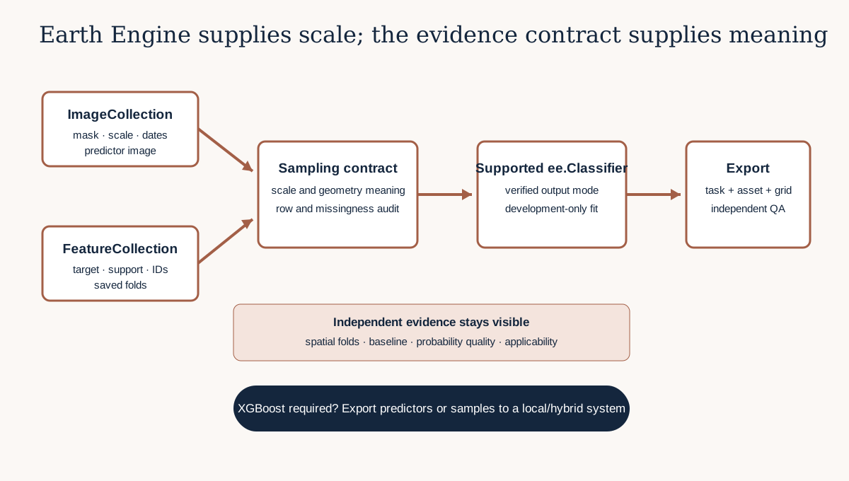
The terracotta gates are decisions that must remain inspectable outside the map display. The large archive is an input advantage. It is not validation evidence.

5. Build the predictor image deliberately

A predictor image should contain only frozen, operationally available features. Its bands must have stable names matching the feature schema. For Sentinel-2, verify whether the chosen collection stores scaled integers and whether your transformations expect reflectance or raw digital values. Masking must be documented because cloud, shadow, snow and edge rules alter which population of pixels remains.

Choose a temporal composite that matches the target's temporal support. A median over an entire growing season and an image within three days of field measurement answer different questions. If training samples use near-date images but deployment uses annual medians, you have created training-serving skew even when band names match.

Do not call reproject() merely to make the display look convenient. Earth Engine normally determines computation scale from the requested operation. State scale and CRS at sampling and export boundaries where support matters, then verify the exported grid.

6. Worked example — specify the component before entering the Code Editor

Run this safe Python audit in the portfolio notebook. It records the intended Earth Engine component without pretending that the browser notebook is authenticated to Earth Engine.

gee_component = {
    "predictor_bands": ["B2", "B3", "B4", "B8", "NDVI"],
    "temporal_rule": "verified seasonal composite",
    "sampling_unit": "field support at documented scale",
    "classifier": "ee.Classifier.smileRandomForest",
    "output_mode": "REGRESSION",
    "validation": "saved site folds outside sampling",
    "export": "versioned image plus task record",
    "xgboost_native": False,
}
required = {"predictor_bands", "sampling_unit", "classifier",
            "output_mode", "validation", "export"}
missing = required - gee_component.keys()
if missing:
    raise ValueError(f"Incomplete component: {sorted(missing)}")
print(gee_component)

Predict before running

1. Will the audit train a model?
2. Why is xgboost_native explicitly false?
3. Which field connects sampling to measurement support?
4. Would changing output_mode from REGRESSION to PROBABILITY preserve the target claim?

Run the cell only after writing your answers. It should display the dictionary without missing-field error. That result establishes structural completeness, not scientific validity or Earth Engine availability.

Code walkthrough

1. The dictionary captures architecture decisions as inspectable data.
2. predictor_bands fixes order and naming, but a complete implementation must also check source, units and transformations.
3. temporal_rule prevents a convenient composite from silently replacing the trained temporal support.
4. sampling_unit makes field-to-pixel support an explicit design issue.
5. classifier names a supported Earth Engine algorithm, not XGBoost.
6. output_mode declares the semantic output required from that classifier.
7. validation preserves saved site folds rather than treating training accuracy as evaluation.
8. export requires both the spatial product and its job record.
9. xgboost_native prevents an unsupported architectural claim.
10. The set comparison catches missing structural fields before implementation.

7. A bounded Earth Engine script pattern

The implementation should follow this sequence in the Earth Engine Code Editor or an authenticated API environment:

var predictors = seasonalImage.select(featureOrder);
var samples = predictors.sampleRegions({
  collection: fieldSupports,
  properties: ['target', 'site', 'fold'],
  scale: predictionScale,
  geometries: true
});
var model = ee.Classifier.smileRandomForest(300)
  .setOutputMode('REGRESSION')
  .train(samples, 'target', featureOrder);
var prediction = predictors.classify(model, 'prediction');

This pattern is intentionally incomplete. A professional script also asserts required properties, applies verified masks and scaling, separates development from protected assessment, records the seed and parameters supported by the chosen classifier, evaluates held-out records, adds applicability and uncertainty evidence where scientifically supported, and exports the versioned result.

ee.Image.classify() expects the input image to contain every band used by the trained classifier, with matching names. A name match is necessary but not sufficient: the unit, temporal rule and transform must also match your external schema.

8. Select a supported output mode

Earth Engine classifiers can expose modes such as CLASSIFICATION, REGRESSION, PROBABILITY, MULTIPROBABILITY, RAW and RAW_REGRESSION. Support varies by classifier. Consult the current official support table before building the workflow. Do not assume that every algorithm supports every mode.

For a continuous vegetation target, choose a classifier supporting REGRESSION and confirm that the numeric target property is correctly represented. For a binary habitat problem, a class output answers a fixed-decision question, while a probability-like output can support ranking, calibration analysis and a separately frozen threshold. Confirm exactly what the algorithm's probability mode returns; do not label any score “confidence” without a definition and calibration evidence.

Earth Engine does not natively execute an XGBoost model as an ee.Classifier. If XGBoost is essential, use a local or hybrid architecture: create/export predictors or samples in Earth Engine, fit and validate XGBoost in the controlled Python environment, and apply it locally or in another documented serving system. Do not rename a Random Forest as XGBoost because both are tree ensembles.

Check your understandingWhich statement about XGBoost in Earth Engine is accurate?

Choose one answer

It is not a native ee.Classifier; use local or hybrid execution when XGBoost is requiredEvery tree ensemble in Earth Engine is XGBoostA model becomes XGBoost when output mode is REGRESSION

Check answer

9. Sampling is a measurement operation

sampleRegions() turns image bands into properties attached to features. That apparently simple conversion contains scientific choices:

• point versus polygon support;
• pixel-centre inclusion and boundary behaviour;
• nominal scale and projection;
• one row per feature, pixel or reduced polygon statistic;
• masked-pixel removal;
• same-day versus composite imagery;
• duplicate or overlapping supports;
• target property type and missingness;
• retention of site, block, date, fold and observation ID.

If a field plot covers 2 × 2 m and the prediction unit is 10 m, sampling the containing pixel does not make the field value a 10 m wall-to-wall truth. Record the reconciliation and the residual support mismatch.

Check your understandingWhat does `scale: 10` in a sampling call establish?

Choose one answer

A computational sampling scale, not automatic equivalence with field supportThat every field target represents exactly 100 square metresThat sampled pixels are independent

Check answer

Use reduceRegions() when a documented reducer over polygon support represents the design better. But a mean, median or percentile is not neutral: it changes which aspect of within-plot heterogeneity becomes a feature.

10. Validation remains independent of platform

Earth Engine can create training and assessment subsets, compute confusion matrices and export sampled tables. The underlying evidence rules remain those of Chapters 3–5:

• split by the spatial or temporal unit that matches deployment;
• keep preprocessing and selection inside development evidence;
• freeze thresholds before protected assessment;
• preserve observation identifiers and fold assignments;
• report fold-level failure, not only a pooled score;
• compare the same baseline on identical assessment units;
• diagnose probability quality, residual geography and applicability.

Randomly splitting sampled pixels is especially misleading when neighbouring pixels share spectra, management and labels. Millions of pixels do not create millions of independent landscapes. The effective transfer evidence is governed by independent sites, times or regions.

When validation is more flexible and auditable in Python, export the modelling table with stable identifiers and run the protected evaluation locally. This is a hybrid architecture, not a failure to use the cloud.

11. Export is part of the scientific result

A map visible in the Code Editor is not a durable deliverable. Export the image and the metadata required to reproduce it. Record:

• script repository commit and parameter-file version;
• source collection and asset IDs;
• date window and composite rule;
• feature order, scale factors and masks;
• model algorithm, parameters and output mode;
• target definition and units;
• CRS, transform, dimensions, scale and region;
• NoData/mask behaviour and output dtype;
• export task ID, creation time, completion state and destination;
• validation evidence and model-card version.

After completion, open the exported file independently. Compare its CRS, bounds, dimensions, transform, band count, mask, value distribution and checksum with the declared contract. A successful task status means the job ran; it does not prove semantic correctness.

Check your understandingWhat does a completed Earth Engine export task prove?

Choose one answer

The specified computation finished, while semantic and independent spatial QA remain necessaryThe prediction is ecologically correctThe classifier generalises to every region

Check answer

12. Diagnostic check — audit the component at four gates

Create a table with one row for each gate.

Gate	Blocking evidence	Pass evidence
Predictor image	missing band, uncertain scale, changed composite	exact schema plus recorded asset/version
Samples	missing target, undocumented support, fold lost	target and identifiers preserved with counts
Model	unsupported mode, assessment used in training	current support verified; development-only fit
Export	ambiguous grid, failed task, missing record	completed task and independent spatial QA

For each gate, include one deliberately failing synthetic case. Demonstrate that your procedure stops or labels the run review rather than quietly continuing.

13. Common mistakes

Treating the map display as a result

Why beginners make it: the interactive map is immediate and persuasive. Recognition: there is no versioned file, metadata or task record. Fix: export, independently validate and package the product.

Claiming XGBoost runs natively

Why: tree-ensemble names sound interchangeable. Recognition: the script uses an Earth Engine smile classifier while documentation says XGBoost. Fix: name the exact algorithm or select a local/hybrid architecture.

Using training accuracy

Why: .confusionMatrix() is convenient after training. Recognition: the same sampled rows fit and evaluate the model. Fix: preserve spatial/temporal folds and report protected predictions.

Losing masked samples silently

Why: masked image bands can remove features during sampling. Recognition: sampled row counts are smaller than the registry without reason codes. Fix: compare expected and returned IDs, quantify losses and investigate them by site/date/class.

Confusing scale with support

Why: a scale: 10 argument appears to define a 10 m ecological observation. Recognition: field support and target assignment are absent from metadata. Fix: document both computational scale and measurement support.

Exporting with implicit defaults

Why: the task accepts minimal arguments. Recognition: grid identity differs across reruns or cannot be reconstructed. Fix: freeze projection, region, transform/scale and dimensions as appropriate, then validate the output.

14. Guided practice — design one Earth Engine component

1. Copy EARTH_ENGINE_COMPONENT_TEMPLATE.md into your portfolio.
2. Restate the target and prediction unit without changing Chapter 1.
3. List five predictor bands with source, unit, scale factor, mask and temporal rule.
4. Draw the field-support-to-pixel relationship.
5. Choose sampleRegions or reduceRegions and justify it.
6. Preserve observation_id, site, block, date and fold.
7. Select one classifier and verify its required output mode in current official documentation.
8. Write a failing check for a missing band and an unsupported output mode.
9. Define protected validation outside the training sample.
10. Specify the exported raster contract and task record.
11. Run the notebook worked example and attach the completed architecture record.

Do not execute a costly or large export merely to finish the lesson. A bounded synthetic region and schema audit are sufficient for the learning objective.

15. Independent challenge — review three architectures

Prepare short designs for:

1. a regional continuous-target regression using a supported Earth Engine algorithm;
2. a rare-habitat classifier requiring probability evaluation and a frozen decision threshold;
3. an XGBoost experiment using Earth Engine only for predictor preparation and export.

For each, specify server-side and local responsibilities, sampling support, validation unit, output semantics, export deliverables and one unsupported claim. Then choose the most defensible implementation for the Environmental Monitoring Project. Your decision must be based on evidence control and operational constraints, not on which platform sounds more advanced.

16. Scientific interpretation

Earth Engine can make archive-scale predictor construction and mapping feasible. It cannot turn correlated pixels into independent validation sites, infer the ecological meaning of labels, correct target-support mismatch or guarantee transfer to a new year. A model output remains conditional on training evidence, feature construction and represented domain.

If a regional prediction shows a spatial pattern, the supported statement is that the fixed model produced that pattern from the stated predictor stack under the audited workflow. Whether the pattern reflects real vegetation state depends on target validity, held-out evidence, uncertainty, applicability and field verification.

17. Submission

Submit:

• EARTH_ENGINE_COMPONENT.md with all four contracts;
• a bounded .js script or pseudocode with verified asset placeholders clearly marked;
• the sampled-schema and missing-ID audit;
• classifier/output-mode evidence linked to current official documentation;
• a versioned export specification and task-record template;
• the Lesson 3.27 checkpoint in the continuing notebook;
• a 300–450 word architecture interpretation naming what Earth Engine does, what remains local and what the workflow cannot claim.

Do not include credentials, private asset paths or a screenshot as the only method record.

18. Portfolio artifact

Artifact 27 — Earth Engine Modelling Component

This artifact adds a bounded cloud component to the Spatial Prediction Pipeline. It demonstrates that you can use archive-scale computation while preserving target meaning, sample support, validation independence, output semantics and export provenance.

19. Reflection

1. Which Earth Engine objects are server-side proxies?
2. Why is random pixel validation usually weak transfer evidence?
3. What does a successful export task prove, and what does it not prove?
4. When is a hybrid architecture more defensible than an all-cloud workflow?
5. Which target-support decision must remain outside the software platform?

20. Core references

• Google Earth Engine supervised classification guide
• Google Earth Engine ee.Classifier.setOutputMode
• Google Earth Engine ee.Image.classify

Further advanced reading

• Google Earth Engine client versus server guide
• Google Earth Engine exporting images
• Google Earth Engine sampleRegions

21. Tested software versions

The local audit targets Python 3.12.13. Earth Engine is a managed service whose API and algorithm support can change; the classifier-mode table and export behaviour were checked against official documentation dated 2026. Record the API environment and script commit used for an actual run. XGBoost 3.3.0 is used only in the local/hybrid pathway and is not presented as a native Earth Engine classifier.