Feature Selection, Redundancy and Stability

1. Problem — a predictor can look important once and still be unstable, redundant or unusable

Learning outcome

By the end of this lesson, you will be able to distinguish predictive reliance from causal importance; calculate permutation importance on held-out development evidence; explain why correlated predictors divide or mask individual importance; summarise relevance across structured folds; compare a full predictor schema with a scientifically reduced schema inside nested validation; and document feature retention using measurement meaning, stability, acquisition cost and operational availability.

• Lesson type: Feature Relevance and Stability Laboratory
• Estimated time: 210–290 minutes
• Prerequisites: Lesson 3.3 predictor hypotheses, Chapter 3 nested validation, Lesson 3.13 search protocol, and Lesson 3.14 learning dynamics
• Portfolio outputs: feature_stability_report.csv, FEATURE_DECISION_LOG.md, full-versus-reduced outer predictions, and the Lesson 3.15 notebook checkpoint

Why this matters

Remote-sensing workflows often produce many related predictors. Several vegetation indices reuse the same red and near-infrared bands. Texture summaries share pixels and scales. UAV height percentiles arise from one surface distribution. Seasonal composites can represent overlapping phenological windows.

A model may predict well while assigning unstable relevance among such variables. One site may favour NDVI, another NDMI, and a third a canopy-height percentile. Removing every correlated variable by an automatic rule can discard complementary measurement information. Keeping everything can increase cost, fragility and training-serving risk. A single ranking cannot resolve those decisions.

Feature selection is therefore part of the model-selection procedure. It must occur inside development evidence, and the complete selection rule must be assessed outside. The decision combines predictive evidence with the predictor hypotheses written before modelling.

Core lesson: retain predictors because their measurement meaning and transferable contribution are defensible—not because one fitted model placed them at the top of a chart.

Mental model

predictor contract
    ├── meaning and support
    ├── availability and cost
    └── known limitations
              +
fold-level held-out relevance
    ├── magnitude
    ├── variation
    └── correlated alternatives
              ↓
predeclared full vs reduced procedure
              ↓
protected outer comparison and stable schema decision

2. Scientific context — many sensors can describe related canopy properties

The Environmental Monitoring Project’s synthetic predictor set includes optical indices, UAV height summaries and texture. The scientific hypotheses are not interchangeable:

• a greenness index may respond to photosynthetically active vegetation but saturate in dense canopy;
• a moisture-sensitive index may carry canopy-water and background information;
• a height percentile represents vertical structure at a declared support;
• texture may reflect spatial heterogeneity but also illumination, resampling and flight artifacts;
• a deliberately added noise feature should not contribute reproducibly.

Correlations arise because vegetation properties co-vary and because derived predictors share measurements. Correlation does not prove redundancy in every deployment context. Two predictors can be strongly correlated in one season and diverge during drought, senescence or sensor failure. Conversely, two differently named indices can add almost no stable predictive information.

This lesson does not discover causal drivers of biomass or habitat condition. It evaluates how the fitted predictive procedure relies on available variables within represented folds.

3. Concept — feature relevance is conditional

Impurity-based tree importance

Tree ensembles can sum reductions in their split criterion for each feature. These values are fast and available after fitting, but can favour high-cardinality variables, reflect training-specific splits and say little about held-out generalisation. They are not causal effects.

Permutation importance

Permutation importance begins with a fitted model and an evaluation dataset. It records a reference score, randomly shuffles one feature column, predicts again, and measures how much the score deteriorates. Repeating the shuffle gives a distribution rather than one number.

For MAE represented by scikit-learn’s negative-MAE scorer, an importance value indicates loss of score after disruption. A larger positive value means the model relied more on that feature for that dataset and metric. A near-zero value can mean the feature is unused, redundant with another feature, weak under that fold, or evaluated in a poor model. A negative value can arise through sampling noise or because disrupting the feature accidentally improves the score.

Permutation importance is conditional on:

• the fitted model and its hyperparameters;
• the training evidence used to fit it;
• the evaluation evidence;
• the chosen metric;
• the other available predictors;
• the permutation scheme and random seed.

It is not an intrinsic property of a Sentinel-2 band, UAV product or ecological process.

Check your understandingWhat does held-out permutation importance measure?

Choose one answer

How much this fitted model's selected score degrades when one feature is disrupted on that evidenceThe causal effect of the environmental variableA universal property of the sensor band

Check answer

4. Visual explanation — stable evidence is a pattern across folds

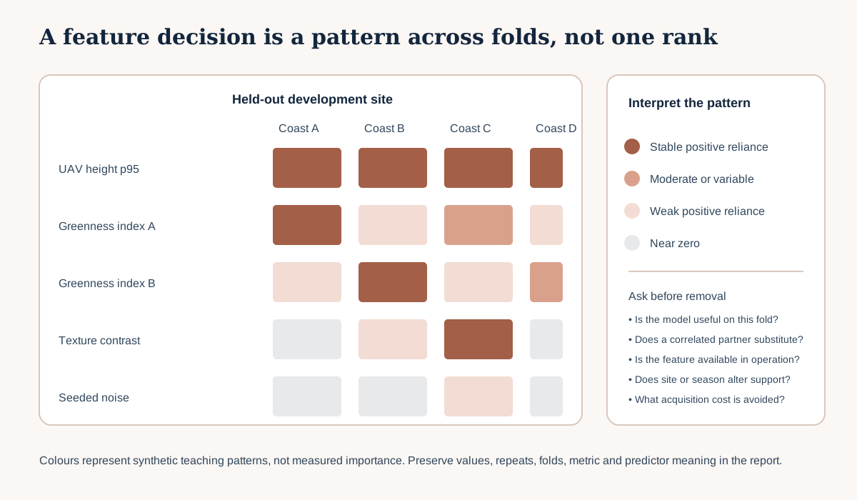
Rows are predictors and columns are structured folds. A consistently positive row indicates repeatable reliance in represented transfer contexts. A patchy row signals site dependence or instability. Two alternating rows may be correlated substitutes: when one is used, the other appears less important. A noise row should hover around zero, but random variation can still produce an isolated positive cell.

Do not compress the matrix into one ranking before inspecting the pattern. Report mean, spread, positive-fold fraction, rank variation and the folds where behaviour changes.

5. Correlated predictors — why individual shuffling can understate a useful group

Suppose NDVI and another greenness index carry very similar information. When NDVI is shuffled, the model may still recover that information from the companion index. NDVI’s individual importance falls. Shuffling the companion produces the same effect. A naive chart concludes that neither matters even when the model depends strongly on their shared signal.

This is not a defect unique to permutation importance. Correlated predictors make individual attribution ambiguous. Options include:

• inspect the correlation structure within each training fold;
• define scientifically meaningful feature families;
• compare a full schema with one representative from a correlated family;
• use grouped permutation as an advanced diagnostic;
• test stability under different represented sites or seasons;
• retain both when they provide complementary operational resilience, while documenting interpretation limits.

Scikit-learn demonstrates clustering correlated variables and selecting a representative, but that is one strategy, not a universal rule. A correlation threshold is a design choice. If chosen from target performance, it belongs inside model selection. If chosen from measurement reasoning, document the reasoning and confirm the schema still serves prediction.

Check your understandingTwo predictors carry similar information. Why can each receive low individual permutation importance?

Choose one answer

The unpermuted partner can retain much of the same predictive informationBoth variables must be measurement errorsCorrelation guarantees neither is useful

Check answer

6. Worked example — held-out permutation relevance inside development

Predict before running

fitted_inner_model was trained on inner-training blocks. X_inner_validation contains a disjoint development block. If two features are strongly correlated, must the lower-ranked one be deleted? Does a large importance prove that changing the environmental variable would change the target? May this inner result be called outer performance?

from sklearn.inspection import permutation_importance

result = permutation_importance(
    fitted_inner_model,
    X_inner_validation,
    y_inner_validation,
    scoring="neg_mean_absolute_error",
    n_repeats=30,
    random_state=42,
)
fold_importance = (
    pd.DataFrame({"feature": X_inner_validation.columns,
                  "importance": result.importances_mean,
                  "spread": result.importances_std})
    .sort_values("importance", ascending=False)
)
fold_importance

Code walkthrough

1. permutation_importance works with a fitted estimator and a chosen evaluation table.
2. The model has seen inner training but not this validation block during fitting.
3. Feature columns must match the saved schema and order.
4. Validation targets calculate the reference and shuffled scores; this makes the result development evidence.
5. The scorer matches the primary selection metric used in the chapter.
6. Thirty repeats reveal permutation variability. They do not create thirty independent sites.
7. The random seed makes the shuffle sequence reproducible.
8. A table binds feature names to mean deterioration and repeat spread.
9. Sorting makes inspection convenient but does not turn ranks into scientific truth.
10. The complete unsorted values and fold identifier should still be saved.

Run the code separately for each structured inner or protected diagnostic fold according to its evidence role. Do not calculate importance on the sealed final test and then alter the feature schema.

Diagnostic check

Before interpreting importance, confirm the model performs better than its baseline on the evaluation fold. Importance from a failing model is not useful evidence of which predictors can support a good model. Then verify:

• feature names and transformations match training;
• the evaluation block did not fit the model;
• metric direction is interpreted correctly;
• repeats are saved, not only means;
• correlation is calculated from the relevant training role rather than all data;
• the noise feature does not appear stably useful;
• every result carries model, fold, schema and seed versions.

7. Stability across folds

For each feature, create a fold-level record with:

• mean permutation importance;
• standard deviation across repeats;
• positive, zero or negative direction;
• rank within the fold;
• model skill on that fold;
• correlated feature family;
• missingness and acquisition availability notes.

Summarise the number and fraction of folds with positive relevance, but keep the raw fold table. A feature positive in four of four outer-development contexts is more stable than one positive in one of four, provided the underlying model has credible fold skill. Still, four sites are only four independent contexts; do not convert the fraction into a population probability.

Rank stability can be assessed descriptively, but rank alone discards magnitude. Features whose importances swap first and second while remaining strong may be practically stable. A feature that falls from a clear positive value to zero in one site requires investigation of range, missingness, season and measurement support.

Check your understandingA feature ranks first in one site fold and near zero in three others. What should the report say?

Choose one answer

Its relevance is unstable across represented transfer contextsIt is the universally best predictorDelete the three inconvenient folds

Check answer

8. Domain-driven selection and a feature decision ledger

Return to the Lesson 3.3 predictor hypotheses. For every candidate feature, record:

1. Measurement meaning: what observable or derived property is represented?
2. Operational availability: can it be produced at prediction time with the same definition?
3. Spatial and temporal support: does it match the prediction unit and date window?
4. Predictive evidence: how does held-out relevance vary across folds?
5. Redundancy: which predictors share bands, pixels, algorithms or ecological response?
6. Cost: what acquisition, storage, licensing, processing or failure burden is introduced?
7. Risk: could missingness, calibration or sensor transition create training-serving skew?
8. Decision: retain, remove, group for comparison, or defer pending evidence.

A feature with modest predictive importance may still be retained if it is inexpensive, stable and safeguards a known seasonal weakness. A high-ranked feature may be rejected if it is unavailable during deployment or derived after the target observation. Predictive performance cannot make an impossible predictor operational.

9. Compare full and reduced schemas without contaminating assessment

Define two or at most a few fixed alternatives:

• Full schema: all predictors that passed the original contracts.
• Scientifically reduced schema: representatives selected through documented measurement reasoning and development-only stability evidence.

Treat schema choice as part of the inner procedure. In each outer fold, select or compare schemas using the current outer development data only. Then refit the chosen procedure and predict the outer assessment once. Preserve which schema was selected and why.

Compare:

• outer MAE and baseline skill by site;
• fold variability and worst-site performance;
• number of predictors and compute time;
• training-serving availability;
• missingness burden;
• selection stability;
• scientific interpretability without causal language.

If the reduced schema performs equivalently within fold variation, it may offer a more robust operational contract. If performance declines materially in particular sites, investigate which measurement information was removed. Do not claim that fewer features are inherently more scientific.

10. Model clinic — four misleading feature-selection stories

“The top feature causes vegetation change”

The model relies on an index for prediction, but management, phenology and canopy structure can jointly affect both index and target. Predictive reliance does not identify an intervention or mechanism. Use causal designs for causal questions.

“Correlation above 0.8 means delete one”

The threshold is imported without checking sensor meaning, seasons or transfer contexts. Correlation may change across domains, and two variables may differ in availability or robustness. Use the threshold as a diagnostic prompt, not an automatic scientific law.

“Zero importance means useless”

The model is poor, or a correlated partner supplies the same information. Check baseline skill, correlated groups and alternative schemas before deciding.

“Importance on the final test confirms the feature set”

The final test is inspected and low-ranked features are removed. It has now influenced model development. Preserve the result as exploratory and obtain new independent evidence for the revised schema.

11. Common mistakes

Calculating importance on training data only

Why beginners make it: the fitted table is immediately available. Recognition: importance is large for a noise or high-cardinality feature. Fix: calculate on appropriately held-out development evidence and first confirm model skill. Consequence: training-specific reliance is mistaken for transferable relevance.

Selecting globally before cross-validation

Why: feature selection feels like preprocessing. Recognition: one reduced table is created using every target. Fix: fit target-informed selection inside inner folds or freeze a domain-driven schema independently. Consequence: outer assessment influences the representation.

Ignoring correlated feature families

Why: importance charts list variables separately. Recognition: all members look weak despite strong model performance. Fix: inspect correlation and compare meaningful groups or representatives. Consequence: useful shared signal can be removed arbitrarily.

Counting repeats as independent folds

Why: thirty permutations produce thirty values. Recognition: uncertainty is reported as though thirty sites were sampled. Fix: separate shuffle variability from variation across independent groups. Consequence: evidence precision is overstated.

Changing the schema without changing its version

Why: removing a column seems minor. Recognition: model files share a name while feature order differs. Fix: version the schema, model, data and decision log together. Consequence: inference can silently receive the wrong features.

Interpreting rank without units or metric

Why: bar charts hide the scorer. Recognition: “importance 0.4” has no stated meaning. Fix: name the score deterioration, evaluation role and target unit. Consequence: results cannot be compared or scientifically interpreted.

12. Guided practice — build the feature stability report

1. Add ## Lesson 3.15 — feature stability to the cumulative notebook.
2. Load the frozen predictor hypotheses and current full schema.
3. Add one seeded synthetic noise predictor only for the diagnostic, clearly label it, and exclude it from any real claim.
4. Fit the selected Chapter 4 procedure inside the current development roles.
5. Confirm credible baseline skill before interpreting importance.
6. Calculate permutation importance on each structured validation fold with thirty repeats.
7. Save repeat-level and fold-summary tables.
8. Calculate training-fold predictor correlations and identify shared-measurement families.
9. Produce the fold-by-feature stability matrix with accessible labels.
10. Complete FEATURE_DECISION_LOG.md for every predictor.
11. Define the full and scientifically reduced schema before outer comparison.
12. Compare both through the nested procedure using identical outer rows.
13. Report performance, stability, cost, missingness and availability.
14. Save feature order and schema hash with each model.
15. Confirm no outer assessment or final-test result was used to revise the reported schema.

13. Independent challenge — an index family under seasonal shift

The supplied synthetic fixture shows two optical indices that are highly correlated in early-season folds but less correlated later, plus a stable UAV height predictor, a site-specific texture predictor and noise.

Prepare a feature decision for two hypothetical deployments:

• satellite-only monitoring across all represented sites;
• combined UAV and satellite monitoring at sites with annual flights.

For each deployment, propose a full and reduced schema. Explain how availability changes the decision, which correlated variables should be compared as a family, what fold evidence is unstable, and what new season or site evidence you would collect. Do not call the highest-ranked variable a cause.

14. Scientific interpretation

Fold-level stability supports a bounded claim about predictive reliance across represented development contexts. A consistently useful canopy-height feature can be described as a stable contributor to this fitted procedure under these folds. It cannot be described as the ecological cause of the target.

Instability may reveal domain differences, correlated substitution, limited groups, measurement noise, preprocessing variation or a genuine shift in which observations carry information. The appropriate response is diagnosis and transparent schema comparison—not deleting inconvenient values.

A professional feature set is a versioned measurement contract. Its value lies in reproducible meaning and operational reliability as well as predictive score.

15. Submission

Submit:

• the executed Lesson 3.15 notebook checkpoint;
• repeat-level permutation results and feature_stability_report.csv;
• an accessible fold-by-feature stability figure;
• the predictor correlation/family audit;
• FEATURE_DECISION_LOG.md;
• full-versus-reduced outer prediction and metric tables;
• the chosen versioned feature schema with order and hash;
• a 400–600 word interpretation that separates predictive reliance from causal explanation.

Portfolio artifact

Feature Stability Report — Chapter 4, Part 3

The report adds a defensible feature schema to the tuning and learning-dynamics records. Lesson 3.16 will apply the same evidence discipline to classification decisions: the model can estimate rare-habitat scores, but the action threshold must be selected from ecological consequences inside development evidence.

16. Reflection

1. Why can two useful correlated predictors each look unimportant?
2. What does permutation importance depend on?
3. Which feature would you retain for operational reliability despite modest mean importance?
4. What would a stable noise-feature importance make you audit?
5. How is a predictive feature decision different from a causal conclusion?

17. Core references and advanced reading

Core references

• scikit-learn 1.9 — permutation feature importance
• scikit-learn — permutation importance with multicollinear or correlated features
• scikit-learn — common pitfalls and data leakage

Optional advanced reading

• scikit-learn — feature selection
• Molnar — Interpretable Machine Learning: permutation feature importance
• Roberts et al. (2017) — cross-validation for structured data

Tested software versions

Python 3.12.13; JupyterLab 4 / Notebook 7; NumPy 2.4.2; pandas 2.2.3; scikit-learn 1.9.0; XGBoost 3.3.0. Stable documentation may advance beyond this tested stack. Record the scorer, model version and feature schema whenever importance is recalculated.