Early Stopping, Regularisation and Learning Dynamics

1. Problem — more boosting rounds can improve training fit after transferable learning has stopped

Learning outcome

By the end of this lesson, you will be able to read training and structured-development loss histories together; distinguish underfitting, overfitting and controlled learning dynamics; explain how learning rate, tree count, tree capacity and regularisation interact; configure XGBoost early stopping without exposing outer assessment; preserve fold-specific best_iteration values; and design a transparent refit rule for the Environmental Monitoring Project.

• Lesson type: Learning Dynamics and Early-stopping Laboratory
• Estimated time: 220–300 minutes
• Prerequisites: Lesson 3.7 XGBoost mechanism, Lesson 3.12 nested evidence roles, and Lesson 3.13 controlled search protocol
• Portfolio outputs: learning_dynamics.csv, LEARNING_DYNAMICS_REPORT.md, three diagnostic figures, and the Lesson 3.14 notebook checkpoint

Why this matters

Boosting is sequential. Each new tree tries to improve the current prediction under the training objective. Given enough capacity, the ensemble can continue fitting small details in the training observations—including measurement noise, site-specific relationships and artifacts of the sampled blocks. A lower training loss therefore does not automatically mean a more useful remote-sensing model.

Early stopping monitors a separate development set and records the round after which its chosen metric no longer improves for a declared patience period. This can save computation and limit unnecessary capacity. It cannot create independent evidence, diagnose every form of leakage, or guarantee transfer to new sites. The monitoring set participates in model selection and must remain inside the current outer development partition.

Core lesson: read learning as a relationship between two evidence streams; never let the protected assessment stream become the steering signal.

Mental model

inner training group → fits tree 1 → tree 2 → ... → tree n
                          ↓         ↓              ↓
training loss          usually decreases
stopping-group loss    improves, plateaus, may worsen
                                      ↑
                         best_iteration is selected here

outer assessment site → used later, once, to assess the complete rule

2. Scientific context — when a meadow model learns one site too closely

The project combines spectral, canopy-height and texture predictors to estimate a declared vegetation target. Relationships can vary with site, phenology, management, soil background, flight conditions and processing. A deep, long-running ensemble may represent the development sites extremely well while relying on interactions that do not transfer.

The practical uses synthetic evidence because its learning patterns are safe to manipulate. You will intentionally create three behaviours:

1. an underfit candidate that cannot improve much beyond the baseline;
2. an overfit candidate whose training loss continues down while structured-development loss deteriorates;
3. a controlled candidate whose capacity and stopping rule produce a smaller and more stable gap.

The purpose is diagnosis, not a beauty contest. A smooth curve does not prove ecological validity. The target contract, predictor availability, grouped folds and final-test firewall remain unchanged.

3. Concept — three different curves answer three different questions

The phrase “learning curve” is used loosely. Separate these designs.

Loss by boosting round

XGBoost’s evaluation history records a metric after each boosting round for the datasets in eval_set. The horizontal axis is ensemble size. This curve answers: as more trees are added, how does fit change on the monitored data? It is the main curve used for early stopping in this lesson.

Learning curve by training-set size

Scikit-learn’s learning-curve tools fit models using increasing amounts of training data. The horizontal axis is number of observations or groups. This asks: would more training evidence plausibly reduce error or the train–validation gap? With spatial data, each size and fold must respect groups; randomly adding neighbouring pixels can produce a misleading answer.

Validation curve by one hyperparameter

A validation curve varies one hyperparameter and compares training with validation performance. It asks: how does a particular capacity control change bias and variance under the selected folds? It is useful for diagnosis but is itself development evidence.

Do not label all three simply “model performance over time.” State the x-axis, metric, unit, data role and grouping.

4. Visual explanation — diagnose the gap, not one line

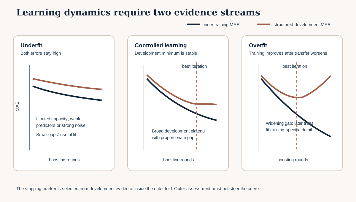
In the underfit panel, both curves remain high and close. The model cannot represent enough useful structure, predictors lack signal, regularisation is too strong, or the target is noisy. A small gap is not automatically good when both errors are poor.

In the controlled panel, training and development loss improve, then the development curve reaches a broad minimum. The gap is present but proportionate to the baseline and fold variation.

In the overfit panel, training loss continues falling while development loss rises. Additional trees improve memorisation of the training partition without improving the monitored transfer task.

The vertical stopping marker is selected from development evidence. It must never be positioned by looking at outer assessment.

Check your understandingTraining MAE keeps falling while structured-development MAE rises. What is the strongest diagnosis?

Choose one answer

Additional capacity is fitting development-specific detail rather than improving transferThe model is necessarily causalThe validation group should be added to training immediately

Check answer

5. Capacity, regularisation and the learning-rate/tree-count trade-off

Early stopping works within a capacity system. It should not be treated as a substitute for understanding the main controls.

Learning rate and tree count

learning_rate scales each new tree’s contribution. A smaller value often needs more boosting rounds, can make learning more gradual, and costs more computation. A very small value is not automatically safer if the model is allowed thousands of rounds and flexible trees. A large value can overshoot stable improvements or reach its minimum quickly.

Tree depth and child evidence

max_depth limits within-tree interaction complexity. min_child_weight makes new child partitions require more accumulated evidence. Deep trees with permissive children can fit small, site-specific groups. Shallow trees can under-represent genuine nonlinear relationships.

Row and feature subsampling

subsample and colsample_bytree introduce stochastic variation and can reduce reliance on particular observations or predictors. They also increase run-to-run variation if seeds are not fixed and do not repair biased sampling.

Leaf penalties

reg_lambda applies an L2-style penalty and reg_alpha an L1-style penalty to leaf weights. gamma requires a minimum loss reduction before a split. Their effects depend on the objective, scale and other settings. Record direction and rationale rather than describing one value as “regularised” in isolation.

Early stopping

early_stopping_rounds=40 means training may continue until the monitored metric has failed to improve for forty consecutive rounds. It is a patience rule, not a fixed tree count. The returned scikit-learn estimator records best_iteration, and its prediction methods use that best iteration automatically in current XGBoost behaviour. Record the installed version because interfaces evolve.

6. Worked example — a stopping group inside outer development

Predict before running

The current outer assessment is coast-d. The remaining development blocks have been divided into X_inner_train and one structurally separated X_stopping_group. If the stopping group’s minimum occurs at round 186, which evidence chose 186? May coast-d appear in eval_set? Should 186 be assumed for every outer fold?

from xgboost import XGBRegressor

model = XGBRegressor(
    n_estimators=2000,
    learning_rate=0.03,
    max_depth=3,
    min_child_weight=3,
    subsample=0.8,
    colsample_bytree=0.8,
    early_stopping_rounds=40,
    eval_metric="mae",
    random_state=42,
    n_jobs=1,
)
model.fit(X_inner_train, y_inner_train,
          eval_set=[(X_inner_train, y_inner_train),
                    (X_stopping_group, y_stopping_group)], verbose=False)

Code walkthrough

1. XGBRegressor supplies the scikit-learn estimator interface.
2. A generous n_estimators ceiling gives early stopping room to identify a development minimum; it is not the intended final tree count.
3. The small learning rate makes updates gradual and must be interpreted with that ceiling.
4. Depth and child weight constrain local interaction capacity.
5. Row and column subsampling add regularisation with a recorded seed.
6. Forty rounds define patience after the best monitored result.
7. MAE matches the predeclared primary error and target units.
8. One thread keeps this teaching run predictable; production resources require a separate compute record.
9. .fit sees only the current inner-training and stopping groups.
10. The first evaluation set allows comparison with training loss.
11. The last evaluation set is the stopping signal under current XGBoost conventions.
12. verbose=False suppresses console output but does not discard evals_result().

After fitting, save model.evals_result(), model.best_iteration and model.best_score. Do not use the outer assessment as the stopping group. XGBoost does not create this split for you; its documentation explicitly places split responsibility on the practitioner.

Diagnostic check

Assert that stopping-group IDs, spatial blocks and sites are disjoint from inner training as required by the declared design. Confirm both sets belong to outer development. Save:

• outer fold and inner split identifiers;
• training and stopping-group MAE for every round;
• best iteration and score;
• patience and upper round limit;
• candidate parameters and seed;
• stopping-group site/block composition;
• any difference between the best round and the final executed round.

Plot the curves with direct labels, target unit and a marker at the selected round. Do not truncate the y-axis to exaggerate a small difference.

Check your understandingMay the outer assessment site serve as XGBoost's early-stopping eval_set?

Choose one answer

No; the stopping round would be selected from assessment evidenceYes; eval_set never changes a modelOnly when MAE improves

Check answer

7. A deliberate three-run diagnostic

Use the same inner evidence and predictor schema for all three runs.

Underfit run

Use very limited capacity, for example shallow trees, high child-evidence requirements and a conservative round ceiling. Predict beforehand whether both losses will remain near the baseline. If performance is poor, do not immediately add complexity: confirm the target, predictors and split are correct.

Overfit run

Use deliberately excessive capacity, such as deeper trees, permissive children and weak subsampling. Keep this bounded to the synthetic fixture. Observe whether training MAE continues downward after development MAE turns. The purpose is to recognise the pattern, not to promote the settings.

Controlled run

Use the Lesson 3.13 selected region with early stopping and recorded regularisation. Compare the best development MAE, train–development gap, best iteration and curve stability.

Place the three results in one table. “Controlled” does not mean “true”; it means the observed learning dynamics are more proportionate under this development design. Outer folds later assess the complete rule.

8. Early stopping inside cross-validation is a procedure, not one command

General cross-validation utilities clone an estimator and call .fit, but XGBoost’s eval_set must be supplied explicitly. A global stopping set reused across folds leaks its information into every candidate. A fold’s validation rows can guide stopping, but then they are selection evidence and cannot simultaneously be described as untouched assessment.

A defensible nested procedure can:

1. create a stopping group inside each current outer development partition;
2. choose parameters and stopping behaviour using only development roles;
3. record fold-specific best iterations;
4. evaluate the resulting procedure on the outer assessment fold;
5. after procedure selection, define a refit rule using development evidence only.

XGBoost’s current documentation notes that early stopping can produce a different number of trees in each cross-validation fold and recommends retraining after cross-validation with selected hyperparameters and early stopping. This is not a licence to use the final test as eval_set. The refit monitoring evidence must still come from development.

9. Decide how to refit without inventing a hidden rule

Fold-specific best iterations might be 140, 186, 225 and 390. Several legitimate development rules are possible:

• rerun early stopping on a dedicated, documented development stopping group;
• use a robust summary such as the median fold best iteration, if predeclared and justified;
• select a conservative value from a plateau, not the absolute most favourable point;
• retain fold-specific fitted models for an explicitly designed ensemble.

Each choice changes the final procedure. Record it before outer or final-test inspection. Do not select the largest number because it “uses more learning,” or the smallest because it “must generalise.” Inspect the curves and site composition.

If best iterations vary widely, report instability. It may reflect different site difficulty, noisy stopping groups, interactions between learning rate and capacity, or too few independent groups. More precise tuning cannot substitute for more representative evidence.

Check your understandingWhy record best_iteration for every structured fold?

Choose one answer

Stopping behaviour may vary by site or block and needs a transparent final refit ruleThe largest number is always the final answerIt proves the model will generalise everywhere

Check answer

10. Model clinic — what the curves do not tell you

Low and parallel curves after leakage

Training and development losses look excellent because derivative pixels from the same plot appear in both roles. The curves diagnose the contaminated split, not real transfer. Re-run the Chapter 3 overlap audit.

A rising development curve caused by domain shift

The stopping group represents one unusual management regime. Early stopping limits fitting but cannot make its predictor range represented in training. Report domain support and investigate in Chapter 5.

A noisy minimum chosen too literally

The curve fluctuates by hundredths of a centimetre and the “best” round changes with a seed. Treat the result as a plateau, report variability and prefer a stable rule. Measurement precision may not support the displayed decimals.

Training metric and scientific metric differ

The objective may optimise squared error while early stopping monitors MAE. That can be reasonable, but document both jobs. Do not assume a lower objective automatically improves every decision metric.

Early stopping after tuning on the same stopping group

Many hyperparameters and the stopping round are repeatedly adapted to one small group. This creates selection pressure even without outer leakage. Use nested roles, constrain flexibility, and assess the complete procedure outside that group.

11. Common mistakes

Using outer assessment in eval_set

Why beginners make it: the API calls it a validation set. Recognition: outer IDs appear in the fit call. Fix: create a stopping role inside outer development. Consequence: outer performance has selected ensemble size and is no longer neutral assessment.

Looking only at validation loss

Why: early stopping prints one monitored series. Recognition: no training curve or gap is reported. Fix: save both histories. Consequence: underfit and overfit patterns can be confused.

Assuming early stopping guarantees no overfitting

Why: the name sounds protective. Recognition: leakage, unrepresentative groups or broad hyperparameter selection are ignored. Fix: treat it as one capacity-control decision inside the full evidence design. Consequence: a contaminated or narrow development set can still produce a misleading model.

Comparing runs with different folds

Why: each notebook cell creates a new random split. Recognition: observation IDs differ among curves. Fix: reuse the saved structured registry. Consequence: model settings and evidence difficulty are confounded.

Recording only the best round

Why: it is compact. Recognition: no metric history or patience is saved. Fix: export every round and the complete fitting metadata. Consequence: reviewers cannot distinguish a broad plateau from a single noisy minimum.

Treating regularisation as an ecological prior

Why: penalties seem like substantive constraints. Recognition: a leaf penalty is described as proof of ecological simplicity. Fix: describe statistical behaviour and keep ecological hypotheses in the predictor register. Consequence: algorithmic constraints become unsupported scientific explanations.

12. Guided practice — build the learning-dynamics report

1. Add ## Lesson 3.14 — learning dynamics to the cumulative notebook.
2. Reuse one saved outer development partition and its inner group registry.
3. Reserve a documented stopping group without using outer assessment.
4. Fit the deliberately underfit configuration and save both metric histories.
5. Fit the deliberately overfit configuration on exactly the same rows.
6. Fit the controlled configuration from the Lesson 3.13 region.
7. Convert the histories to tidy learning_dynamics.csv with run, fold, dataset role, round and MAE.
8. Plot all three runs with accessible labels and consistent axes.
9. Mark each best iteration and report patience.
10. Compare best development MAE with the Chapter 2 baseline.
11. Repeat the controlled procedure across outer folds without reusing outer assessment as stopping evidence.
12. Summarise variation in best iterations and performance.
13. Declare the refit rule and version it.
14. Confirm the final-test access log is unchanged.
15. Write limitations concerning few groups, synthetic evidence and the distinction between algorithmic learning and ecological mechanism.

13. Independent challenge — review a misleading training report

A colleague submits a figure showing training RMSE decreasing for 2,000 rounds and states, “The model continuously learns more accurate ecology.” No development curve, units, split IDs or baseline are shown.

Produce a review that:

• identifies every unsupported statement;
• specifies the minimum missing evidence;
• proposes a grouped stopping design;
• distinguishes objective, monitored metric and final decision metric;
• explains three possible causes of a widening gap;
• defines a versioned final refit rule;
• states what the resulting evidence would and would not support.

Then use the supplied synthetic learning-dynamics fixture to label each run as underfit, overfit or controlled. Defend each label from both curves and the baseline, not from the run name.

14. Scientific interpretation

A stopping minimum indicates where additional trees ceased to improve the selected metric on a particular development role. It does not identify the true complexity of coastal-meadow ecology. The best iteration is conditional on predictor schema, objective, metric, grouping, seed, learning rate, regularisation and evidence composition.

Consistent controlled dynamics across several outer development contexts increase confidence that the training rule is stable within the represented domains. Large variation is itself a result and may motivate a simpler rule, larger stopping groups or more independent sites.

The strongest claim remains procedural: the model’s capacity was controlled using development evidence that did not contaminate outer assessment or final testing.

15. Submission

Submit:

• the executed Lesson 3.14 notebook checkpoint;
• learning_dynamics.csv with all three runs and both data roles;
• accessible underfit, overfit and controlled figures;
• LEARNING_DYNAMICS_REPORT.md with curve interpretation and refit rule;
• fold-level best_iteration and best_score records;
• an evidence-role audit proving outer assessment stayed outside eval_set;
• a 400–600 word scientific interpretation with limitations.

Portfolio artifact

Learning Dynamics Report — Chapter 4, Part 2

This report adds a transparent capacity and stopping policy to the Controlled Tuning Protocol. Lesson 3.15 will now ask whether the predictor schema itself is stable across folds, rather than assuming that one fitted model’s feature ranking is a permanent scientific truth.

16. Reflection

1. Why can a small train–development gap still indicate underfitting?
2. What evidence does best_iteration depend on?
3. How does learning rate change the meaning of a tree-count comparison?
4. Which source of domain shift could early stopping not repair?
5. What would wide variation in fold-specific best iterations make you do next?

17. Core references and advanced reading

Core references

• XGBoost — scikit-learn estimator interface and early stopping
• XGBoost parameter reference
• scikit-learn — validation curves and learning curves

Optional advanced reading

• XGBoost callback API
• Chen and Guestrin (2016) — XGBoost
• scikit-learn — common pitfalls

Tested software versions

Python 3.12.13; JupyterLab 4 / Notebook 7; NumPy 2.4.2; pandas 2.2.3; scikit-learn 1.9.0; XGBoost 3.3.0. The XGBoost stable documentation may describe a newer version than the Academy’s tested environment, so verify constructor, callback and prediction behaviour when reproducing the lesson.