Hyperparameter Optimisation

1. Problem — optimisation can improve a procedure or merely exploit its validation evidence

Learning outcome

By the end of this lesson, you will be able to distinguish a model parameter from a learned parameter; design a small, scientifically motivated hyperparameter search space; run reproducible RandomizedSearchCV inside grouped development folds; preserve Chapter 3’s outer-assessment and final-test firewalls; inspect the complete search record rather than one winning score; and compare an untuned procedure with a tuned procedure on identical protected evidence.

• Lesson type: Controlled Search Design Laboratory
• Estimated time: 210–290 minutes
• Prerequisites: Lessons 3.1–3.12, especially the frozen experiment plan, baseline, first XGBoost candidate and nested grouped-validation design
• Portfolio outputs: TUNING_PROTOCOL.md, search_results.csv, outer_tuned_predictions.csv, and the Lesson 3.13 checkpoint in Environmental_Monitoring_Project_Starter.ipynb

Why this matters

XGBoost exposes many settings. Software makes them easy to vary, but a large menu is not a scientific reason to search. Every additional candidate consumes computation and gives chance another opportunity to fit peculiarities of the development folds. If the same evidence chooses a candidate and is then reported as neutral assessment, the result exaggerates what has been learned.

Hyperparameter optimisation is therefore an experimental design problem. You must define what may change, why each range is plausible, which evidence may choose among candidates, what metric represents the scientific error, and how much search is proportionate to the number of independent sites or blocks. A search result is defensible only when its evidence role is traceable.

Core lesson: optimise the complete modelling procedure inside development evidence; assess that procedure on evidence that could not influence the choice.

Mental model

scientific rationale
        ↓
bounded candidate space + fixed budget + fixed seed
        ↓
inner grouped folds choose a procedure
        ↓
refit on current outer development partition
        ↓
outer site assesses the selection procedure once
        ↓
repeat for every outer fold; final test remains sealed

The object being evaluated is not one lucky parameter dictionary. It is the declared rule for producing a model from new development data.

2. Scientific context — improve the coastal-meadow predictor without changing the claim

The Environmental Monitoring Project still predicts the target and prediction unit specified in Chapter 1. The predictor meanings, spatial support, valid rows and baseline also remain fixed. Chapter 3 established a primary new-site transfer design: outer sites assess the complete procedure, while spatial blocks inside the remaining sites provide inner selection evidence.

Lesson 3.13 is allowed to compare a restrained set of XGBoost behaviours. It is not allowed to:

• change the target after seeing search results;
• add predictors because they correlate with outer residuals;
• select a cloud threshold from an outer site;
• replace grouped inner folds with convenient random rows;
• discard a difficult outer fold;
• open the Academy final test;
• present the best inner score as final performance.

The synthetic training pack is designed to practise these roles. It does not measure Baltic coastal meadows and cannot establish operational accuracy. The real project later uses documented data only after its target, units, sampling and EO provenance pass the earlier contracts.

3. Concept — parameters are learned; hyperparameters define how learning occurs

A fitted tree learns split variables, split thresholds and leaf values from training observations. Those are model parameters. max_depth, learning_rate, min_child_weight, subsample and the number of boosting rounds shape how that learning can happen. They are hyperparameters because the fitting algorithm does not ordinarily determine them from its training objective alone.

Changing a hyperparameter changes model behaviour:

• max_depth limits interaction complexity within each tree;
• min_child_weight demands more accumulated evidence before a child is retained;
• learning_rate shrinks each tree’s contribution and interacts with tree count;
• subsample trains a boosting round on a fraction of rows, adding stochastic regularisation;
• colsample_bytree restricts the predictors offered to a tree;
• reg_lambda and reg_alpha penalise leaf weights in different ways.

The search should include parameters with a plausible role in the observed modelling problem. It should not include everything in the API. A narrow space can still be inadequate, but breadth without evidence is not rigour.

Manual tuning, grid search and random search

Informed manual tuning is useful for understanding large behavioural changes and catching invalid ranges. It becomes difficult to reproduce if choices are made informally after each score.

Grid search evaluates every Cartesian combination in a discrete grid. Three values for each of five parameters produce $3^5 = 243$ candidates before folds are counted. A grid can spend most of its budget varying parameters that matter little while testing only three values of a sensitive parameter.

Random search samples a fixed number of candidate combinations. Its explicit n_iter separates computational budget from the size of the conceptual space. It is often a practical first choice when several parameters may matter. Random search is not random scientific reasoning: ranges, distributions, metric, folds, budget and seed all require justification.

Optional optimisation libraries can propose candidates more adaptively, but they do not repair poor evidence design. This chapter uses RandomizedSearchCV because its selection record and fold behaviour are visible without adding a new optimisation framework.

Check your understandingWhere may RandomizedSearchCV compare hyperparameters during a nested outer fold?

Choose one answer

Only inside the current outer development partitionOn the outer assessment siteOn the sealed final test

Check answer

4. Visual explanation — a search is contained by two evidence firewalls

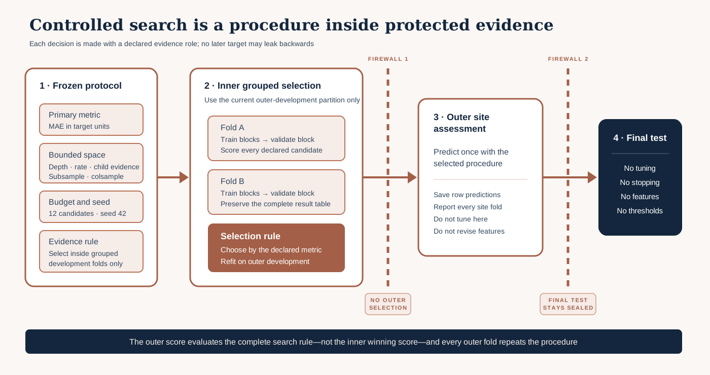
The left side is a design record: candidate ranges, budget, metric and random seed are frozen. The centre is the only place where candidates compete. The first firewall prevents outer-assessment targets from entering candidate choice. The second keeps the final test closed throughout the chapter.

Notice that each outer fold runs a new inner search. That repetition evaluates the full procedure and exposes whether different site contexts prefer different settings. A parameter chosen in every outer fold is more stable than one that wins once, but frequency alone does not prove it is universally correct.

5. Design a search space from behavioural hypotheses

Begin with the Chapter 2 candidate, not an empty canvas. For each proposed range, complete four statements:

1. Behaviour: what aspect of fitting changes?
2. Reason: what evidence suggests this behaviour needs testing?
3. Boundary: why is the minimum and maximum plausible for this dataset and compute budget?
4. Risk: what failure could an extreme value produce?

An example record might state that depths 2–4 test modest nonlinear interactions among canopy height, spectral response and texture. Depth 1 may under-represent plausible interactions; much deeper trees may isolate tiny site-specific groups in a dataset with few independent sites. That is a hypothesis to evaluate, not a guarantee that depth 3 is correct.

For a first controlled search, prefer a small set such as:

Hyperparameter	Candidate values	Behavioural question
max_depth	2, 3, 4	How much interaction complexity transfers across blocks?
learning_rate	0.02, 0.05, 0.10	How cautiously should successive trees update predictions?
min_child_weight	1, 3, 6	How much evidence should a child partition require?
subsample	0.7, 0.9, 1.0	Does row subsampling reduce development-specific fitting?

Do not interpret this table as a universal recipe. Sample size, target noise, predictor support, missingness and deployment domain all matter. Record changes as a new protocol version if initial diagnostics show a range is nonsensical.

Candidate budget

Twelve random candidates across three inner folds require 36 fits for one outer fold, plus refitting. Repeating across four outer sites requires at least 144 candidate fits. That arithmetic belongs in the protocol because computational affordability affects what can be reproduced.

The budget should be chosen before scores appear. If all values are finite lists, scikit-learn samples combinations without replacement. If a continuous distribution is supplied, sampling behaviour differs. Record the exact object, package version and seed—not merely the phrase “random search.”

Check your understandingWhat makes a search space scientifically defensible?

Choose one answer

Each range has a behavioural rationale, feasible budget and predeclared boundsIt contains every value the software acceptsIt is expanded until one score looks impressive

Check answer

6. Worked example — search only the current outer development partition

Predict before running

Assume the current outer assessment site is coast-d. Which rows may enter search.fit? Which grouping variable directs the inner splitter? If the best inner MAE is 3.8 cm, may that value be reported as new-site performance? Write your answers before reading the code.

from sklearn.model_selection import GroupKFold, RandomizedSearchCV
from xgboost import XGBRegressor

inner = GroupKFold(n_splits=3)
search = RandomizedSearchCV(
    XGBRegressor(objective="reg:squarederror", random_state=42, n_jobs=1),
    {"max_depth": [2, 3, 4], "learning_rate": [0.02, 0.05, 0.1],
     "min_child_weight": [1, 3, 6], "subsample": [0.7, 0.9, 1.0]},
    n_iter=12, scoring="neg_mean_absolute_error", cv=inner,
    random_state=42, n_jobs=1, refit=True,
)
search.fit(X_outer_development, y_outer_development,
           groups=block_outer_development)

Code walkthrough

1. The imports provide a grouped splitter and a budgeted random search.
2. GroupKFold keeps each spatial block in one inner role. It must receive groups from the current outer development partition only.
3. The estimator fixes the regression objective, seed and thread count. These are part of reproducibility.
4. The dictionary contains four behaviourally justified dimensions. It is not expanded after seeing the outer assessment.
5. n_iter=12 freezes the candidate budget.
6. Negative MAE follows scikit-learn’s scorer convention that larger values are better. Multiply reported values by −1 when communicating error in centimetres.
7. cv=inner makes selection depend on grouped inner validation, not random rows.
8. The search seed makes the sampled candidate list repeatable under the recorded software version.
9. Keeping search and estimator parallelism at one avoids competing thread pools in the teaching environment.
10. refit=True refits the selected candidate on all current outer development rows after inner comparison.
11. Only outer development features and targets enter .fit.
12. Spatial block labels determine inner separation.

After fitting, use the refitted search object to predict the untouched outer assessment site once. Save those predictions with observation IDs, outer fold, selected parameters and protocol version. Do not use the assessment error to alter the search within that same reported experiment.

Diagnostic check

Export cv_results_ to search_results.csv. For each candidate preserve:

• parameter values;
• mean and standard deviation of inner validation MAE;
• rank under the predeclared primary metric;
• fit time and score time;
• failure or warning status;
• outer fold and search seed;
• exact inner group registry.

Check whether the winner barely differs from several alternatives. A difference smaller than fold variation does not support a dramatic claim. Prefer a simpler candidate when performance is practically equivalent and the simplification was part of the selection rule.

7. Search results are a distribution, not a trophy

The best_params_ attribute is convenient, but it hides the evidence around the winner. Inspect the rank table and fold columns. Ask:

• Does one candidate win because of one favourable block?
• Do nearby parameter values perform similarly?
• Are some combinations unstable or invalid?
• Does deeper capacity improve training score but not inner validation?
• Does the selected parameter pattern change across outer sites?
• Is the compute cost proportionate to any error reduction?

A broad plateau of similar scores often supports a conservative region rather than one magical point. Strongly varying winners may mean the search is noisy, sites differ, inner groups are scarce, or the model is underidentified by current evidence.

Do not average parameter values across folds. A mean depth of 2.75 is not a selected tree depth and may not correspond to any evaluated procedure. Instead, record fold-specific selection and declare how the final development procedure will be chosen after nested evaluation.

8. Compare tuned and untuned procedures fairly

The Chapter 2 candidate is the control. In every outer fold:

1. fit the untuned fixed procedure using outer development only;
2. run the declared inner search on the same outer development rows;
3. refit the selected candidate on those rows;
4. predict the same outer assessment observations with both;
5. calculate the same predeclared metric and baseline skill;
6. preserve paired observation-level errors.

Report fold-level differences, not only two pooled means. Tuning that improves three sites by 0.2 cm but worsens one site by 4 cm is not a uniform improvement. The difficult site may represent a support gap that optimisation cannot solve.

The outer comparison evaluates the procedure “run this bounded search on development data,” not the inner winning score. The sealed final test is not required for this lesson and must remain unopened.

Check your understandingHow should tuned and untuned candidates be compared?

Choose one answer

On identical protected outer folds with the same metric and featuresUsing each model's best inner scoreBy opening the final test for both

Check answer

9. Model clinic — apparently careful searches that still leak

Search after global feature selection

Predictors were ranked using every target before nested validation. Even if RandomizedSearchCV uses inner folds correctly, the feature set already contains outer information. Put data-dependent feature selection inside the inner procedure or use a feature set frozen independently of outer outcomes.

Search with ordinary K-fold inside spatial data

The outer site is protected, but neighbouring blocks are randomly divided inside development. Candidate choice may favour complexity that exploits inner proximity. Use the structured inner unit declared in Chapter 3.

Expanding the space after outer failure

A poor outer site motivates ten new ranges, then all outer results are presented as one neutral estimate. The original outer evidence has influenced development. Preserve version 1 results, label the change as version 2, and recognise that fresh assessment is required for the revised procedure.

Choosing by many metrics after viewing them

MAE, RMSE, R² and bias are computed, and whichever makes the winner look best becomes “primary.” Freeze the primary selection metric and use secondary metrics diagnostically. Chapter 5 will deepen metric interpretation.

Treating failed fits as missing at random

Candidate failures can remove difficult combinations or folds. error_score=np.nan may allow a search to finish but does not make failures irrelevant. Investigate, record and decide whether the candidate space violates valid model constraints.

10. Common mistakes

Searching every available parameter

Why beginners make it: more combinations appear more thorough. Recognition: the protocol contains no behavioural rationale and the fit count grows explosively. Fix: begin from the first defensible candidate and vary only parameters linked to a declared hypothesis. Scientific consequence: flexible selection can fit noise while obscuring what changed.

Using the final test to settle a close result

Why: the final test seems authoritative. Recognition: test error chooses between parameter regions. Fix: use development evidence and a predeclared simplicity rule; open the final test only after the full procedure is frozen. Consequence: final-test independence is lost.

Reporting best_score_ as performance

Why: it is prominently exposed by the API. Recognition: no outer prediction file exists. Fix: report the distribution of protected outer predictions. Consequence: selection evidence is mistaken for assessment.

Forgetting the sign of neg_mean_absolute_error

Why: scikit-learn maximises scorers. Recognition: a report claims that −3 cm is a physical MAE. Fix: convert to positive error for scientific reporting and name the unit. Consequence: results become confusing or incorrectly ranked outside the search object.

Allowing nested parallelism to consume all resources

Why: both tools accept n_jobs=-1. Recognition: memory pressure, thread thrashing or irreproducible runtimes. Fix: parallelise at one level, record resources and test a small run first. Consequence: a technically valid search becomes operationally unreproducible.

Treating the winning values as ecological findings

Why: parameters acquire scientific-sounding interpretations. Recognition: “depth 3 proves three ecological processes.” Fix: describe model behaviour, not causal mechanism. Consequence: an engineering choice is converted into an unsupported ecological claim.

11. Guided practice — produce a controlled tuning record

1. Add ## Lesson 3.13 — controlled hyperparameter search to the cumulative notebook.
2. Copy the target, feature schema, baseline, primary metric and Chapter 3 nested fold identifiers without changing them.
3. Open TUNING_PROTOCOL_TEMPLATE.md and state the purpose of tuning in one sentence.
4. Write a behavioural rationale, minimum, maximum and risk for each searched hyperparameter.
5. Calculate the discrete grid size, even though the practical uses a 12-candidate random budget.
6. Record the candidate budget, expected fit count, seed, thread policy and stop condition for failed candidates.
7. Assert that every outer assessment row is absent from inner search inputs.
8. Run the search separately inside each outer development partition.
9. Export complete cv_results_ with positive MAE reporting columns.
10. Refit and predict each outer assessment fold once.
11. Join tuned and untuned predictions by observation ID and outer fold.
12. Calculate paired MAE differences and baseline skill by site.
13. Describe parameter-selection stability without averaging parameter values.
14. Confirm that the final-test access log remains empty.
15. Write a decision: retain the untuned control, adopt the bounded search procedure, or collect more development evidence.

12. Independent challenge — defend the budget to a scientific review panel

Design two alternative protocols for the same nested evidence:

• a minimal protocol with no more than six candidates;
• a standard protocol with twelve to twenty candidates.

For each, state the parameter hypotheses, candidate count, total expected fits, grouping, metric, compute estimate and failure policy. Use the supplied synthetic search-results fixture to identify a stable performance region. Then argue which protocol is proportionate to four outer sites and a limited number of inner blocks.

Your answer must discuss why a 500-candidate search would not create 500 independent ecological experiments, what evidence would justify expanding the space, and how you would version a second search after learning from the first. Do not choose from outer or final-test performance.

13. Scientific interpretation

If the tuned procedure lowers outer MAE consistently across represented sites, the evidence supports a bounded statement: the declared inner-search procedure improved predictive transfer relative to the fixed untuned candidate under these outer folds. It does not prove that the selected values are optimal, that the model will transfer to a new biome, or that the most influential settings represent ecological mechanisms.

If outer improvement is absent, optimisation has still produced useful knowledge. The initial candidate may already occupy a broad stable region; independent groups may be too few to rank alternatives; predictor or target quality may dominate; or site shift may require better evidence rather than more capacity.

Record uncertainty in model selection itself. Variation in selected parameters and fold outcomes belongs in the scientific result.

14. Submission

Submit:

• the executed Lesson 3.13 notebook checkpoint;
• TUNING_PROTOCOL.md frozen before the search;
• search_results.csv with every candidate and inner-fold score;
• outer_tuned_predictions.csv aligned with untuned predictions;
• one accessible figure comparing paired outer errors;
• the search-space and compute-budget calculation;
• a 400–600 word decision explaining whether controlled tuning improved the procedure and what evidence remained protected.

Portfolio artifact

Controlled Tuning Protocol — Chapter 4, Part 1

This artifact turns Chapter 3’s Structured Validation Design into an executable model-selection procedure. It records the search rationale, budget, complete results, outer predictions and decision. Lesson 3.14 will examine how the selected capacity learns over boosting rounds rather than treating tree count as an arbitrary large number.

15. Reflection

1. Which searched parameter has the clearest behavioural rationale for this target and why?
2. What is the difference between the best inner score and outer evidence?
3. When would a grid be more transparent than random search?
4. What would make a twelve-candidate budget excessive or insufficient?
5. How would you report a different winner in every outer site?

16. Core references and advanced reading

Core references

• scikit-learn 1.9 — RandomizedSearchCV
• scikit-learn 1.9 — tuning estimator hyperparameters
• Cawley and Talbot (2010) — model selection over-fitting

Optional advanced reading

• Bergstra and Bengio (2012) — Random Search for Hyper-Parameter Optimization
• scikit-learn — grouped cross-validation
• XGBoost parameter reference

Tested software versions

Python 3.12.13; JupyterLab 4 / Notebook 7; NumPy 2.4.2; pandas 2.2.3; scikit-learn 1.9.0; XGBoost 3.3.0. The Academy site records the tested environment, while linked stable documentation may describe a newer compatible release. Recheck APIs when reproducing the work.