Spatial Joins, Overlay and Nearest Neighbours

1. Combine spatial evidence without hiding ambiguity

Learning outcome

By the end of this lesson, you will be able to distinguish attribute joins, predicate-based spatial joins, nearest-neighbour joins and overlay; select a relationship that matches the scientific question; retain unmatched features; detect one-to-many outcomes and duplicated identifiers; and produce a cardinality audit before accepting joined data. You will add site, management and vegetation assignments to the synthetic training points without forcing ambiguous cases into one category.

Prerequisites: Complete Lessons 2.5–2.6. You should be able to audit GeoDataFrames, transform layers to a common projected CRS and explain within, contains and intersects. Allow 120–150 minutes.

Why this matters

Spatial joins create tables that can look ordinary enough to analyse immediately. One plot row gains a site name, management regime and vegetation zone; the workflow appears complete. Yet the relationship may be wrong, ambiguous or incomplete.

A point can fall outside every polygon because of positional error, outdated boundaries or genuine sampling outside the mapped area. A point on a shared boundary can match two polygons with intersects or none with within. Overlapping polygons can turn one plot into several output rows. Dropping duplicates or unmatched rows without diagnosis changes the evidence.

Core spatial question: Which spatial relationship should connect these observations, and can one input legitimately match several features?

Scientific context

The vector training pack contains five synthetic plot points:

• three are inside training zones;
• TP04 lies exactly where shared management and vegetation boundaries meet;
• TP05 lies outside the training study area.

These are designed QA cases, not bad data to remove. Your workflow should make each consequence visible. In governed research data, such cases would trigger checks against field protocol, positional accuracy, boundary provenance and acquisition date.

Learner action

Add ## Lesson 2.7 — Spatial joins, overlay and nearest neighbours to the Module 2 notebook. Before running code, create a prediction table for each plot with columns within_match, intersects_match_count and expected_review. Use the README and geometry, not a desired final table.

2. Attribute and spatial joins use different evidence

An attribute join matches rows through a shared key. If a validated site_id exists in both a plot table and a site metadata table, a pandas-style merge may be appropriate. Its credibility depends on key meaning, uniqueness and referential integrity.

A spatial join matches features through a geometric predicate. It is appropriate when the relationship itself is spatial—for example, assigning a point to a polygon that contains it.

Do not replace a trustworthy attribute key with a spatial join simply because geometry is available. Conversely, do not join through similar site names when the intended relationship is containment and names are inconsistent. State which evidence defines the relationship.

Before either join, define expected cardinality:

• one-to-one: each plot should match exactly one zone;
• many-to-one: many plots may belong to one zone;
• one-to-many: one plot can legitimately match several zones;
• many-to-many: several features on each side may relate.

Cardinality is a scientific expectation, not merely a database setting.

Check your understandingA validated site_id exists in both the plot table and site metadata table. What relationship should be considered first?

Choose one answer

A validated attribute join, because the shared key already defines the relationshipA nearest spatial join with no distance limitAn overlay that splits every plot geometry

Check answer

3. Predicate direction must match the left and right layers

For a point-on-left, polygon-on-right join:

plots.sjoin(zones, how="left", predicate="within")

asks whether each left point is within each candidate right polygon.

Reversing the layers changes both the readable question and which geometry is retained. A polygon-on-left join might use contains to ask whether each polygon contains candidate points. Avoid choosing a predicate from memory; write the relationship in a sentence with explicit subject and object.

Important boundary behaviour:

• within requires the point to be in the polygon interior, not only on its boundary;
• intersects accepts any shared spatial portion, including a boundary point;
• covered_by can include boundary membership where that rule is scientifically intended;
• touches identifies boundary-only contact.

Available predicates depend on the spatial-index implementation. Inspect gdf.sindex.valid_query_predicates rather than assuming every environment supports the same set.

4. Join type controls which observations survive

The how argument controls row retention and the active output geometry:

• how="left" keeps every feature from the left GeoDataFrame and retains the left geometry;
• how="inner" keeps only matched left features and retains the left geometry;
• how="right" keeps right-side features and retains the right geometry.

For a first assignment audit, a left join from plots to zones is usually safest because unmatched plot records remain visible. An inner join can silently remove exactly the cases that need investigation.

The output includes right-side attributes and an index reference. Rename fields clearly and retain stable identifiers from both inputs. Do not let automatically suffixed column names become an undocumented data model.

5. One-to-many matches create repeated left identifiers

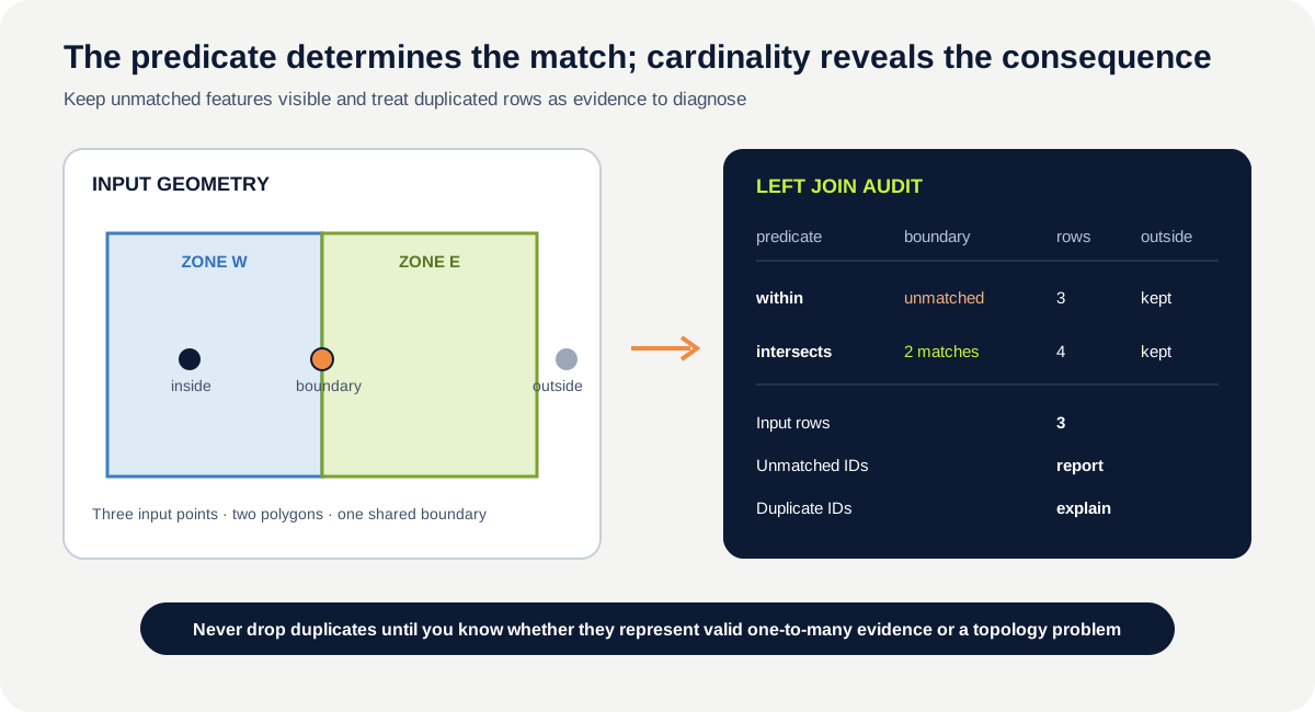
When one point matches two polygons, a spatial join needs two rows to represent both relationships. The geometry and plot_id repeat; the right-side zone identifier differs.

This is not automatically a duplicate-data error. It may reveal:

• a point on a shared boundary;
• overlapping polygons;
• different zone systems represented in one layer;
• a deliberately many-valued relationship;
• topology or positional error.

The correct response is to diagnose first. Never call drop_duplicates("plot_id") until an independently justified rule selects or aggregates the matches.

Check your understandingA left spatial join produces more rows than the input plot layer. What should you do first?

Choose one answer

Identify repeated plot IDs and diagnose legitimate one-to-many matches, overlaps or topology problemsDrop duplicated plot IDs and keep the first rowSwitch to an inner join so the table looks cleaner

Check answer

6. Worked example — audit a management-zone assignment

Before running, predict the input and output row counts. Which plot should remain unmatched with within, and why?

from pathlib import Path
import geopandas as gpd

folder = Path("data/training/vector_foundations")
plots = gpd.read_file(folder / "training_field_plots.geojson").to_crs("EPSG:3301")
zones = gpd.read_file(folder / "training_management_zones.geojson").to_crs(plots.crs)
joined = plots.sjoin(zones, how="left", predicate="within")

audit = {
    "input_rows": len(plots),
    "output_rows": len(joined),
    "unmatched": int(joined["management_id"].isna().sum()),
    "repeated_plot_ids": int(joined["plot_id"].duplicated(keep=False).sum()),
}
print(audit)
print(joined[["plot_id", "management_id"]])

The left join should retain all five input plots. The interior plots receive a management assignment. TP04, on the shared internal boundary, has no within match. TP05, outside the training zones, also remains unmatched. The input and output row counts remain equal for this predicate because no point is within more than one non-overlapping zone.

Code walkthrough

1. Path defines one reproducible training-data folder.
2. GeoPandas is imported with the standard alias.
3. The synthetic plot points are read and transformed to EPSG:3301.
4. The management zones are read and transformed to the exact plot CRS.
5. sjoin evaluates left-point within right-polygon relationships.
6. how="left" preserves unmatched plot geometries for review.
7. audit stores join evidence rather than relying on the displayed table.
8. input_rows records the expected analysis population.
9. output_rows reveals expansion or loss.
10. Missing management_id counts unmatched relationships.
11. duplicated(keep=False) would count all rows participating in repeated plot IDs.
12. The first print exposes summary evidence.
13. The second displays stable identifiers from both sides so individual cases remain traceable.

Now repeat with predicate="intersects". TP04 intersects both management polygons, so it should produce two rows. TP05 remains unmatched. An output row count greater than the input count is expected evidence of a one-to-many boundary case—not a reason to delete a row.

7. Build a cardinality audit for every spatial join

At minimum, record:

Audit field	Purpose
left and right layer names	identifies the relationship inputs
left/right CRS	confirms comparable coordinate space
predicate and how	states the join rule
input row counts	establishes the starting populations
output row count	reveals loss or expansion
unmatched left IDs	preserves unresolved observations
repeated left IDs	reveals one-to-many results
unused right IDs	reveals zones with no assigned observations
geometry retained	prevents mistaken interpretation of output support
decision for ambiguous cases	makes exclusions or multiple membership reviewable

Also check whether right-side identifiers are unique before joining. A duplicated zone record can multiply rows even when geometries are identical.

Compare expected and observed cardinality. If you expected many-to-one and observe one-to-many, stop the downstream analysis until the reason is understood.

8. Nearest is a hypothesis with a distance threshold

sjoin_nearest() matches each left geometry to the closest right geometry. It is useful when proximity—not containment—is the intended relationship. It should not be used merely to eliminate missing values.

Use it only after:

1. transforming both layers to a suitable projected CRS;
2. defining a scientifically defensible maximum distance;
3. requesting a distance column;
4. checking ties and repeated identifiers;
5. retaining cases with no neighbour inside the threshold.

nearest = plots.sjoin_nearest(
    zones,
    how="left",
    max_distance=100,
    distance_col="distance_m",
)

Without max_distance, every point can receive a nearest feature even when the distance is scientifically absurd. For a point already inside a polygon, distance to that polygon is zero. Equal-distance neighbours can create several result rows.

The threshold must come from positional accuracy, sampling design or a process-based rule—not from the distance that produces complete assignments.

Check your understandingWhat makes a nearest-neighbour spatial join scientifically reviewable?

Choose one answer

Projected units, a justified maximum distance, an output distance column and explicit tie/unmatched checksAssigning a nearest feature to every point regardless of distanceRemoving the distance column after the join

Check answer

9. Overlay creates new geometry rather than attaching attributes

Spatial join and overlay are not synonyms.

• Spatial join: retains one side’s active geometry and attaches attributes according to a relationship.
• Overlay: performs set operations between input geometries and returns newly partitioned geometry with attributes from both inputs.

Intersecting management and vegetation polygons creates pieces representing combinations such as west-management × lower-vegetation. Feature count can increase, geometry can fragment and small sliver polygons can appear.

Before overlay:

• ensure a common suitable CRS;
• inspect validity and geometry types;
• define the intended set operation;
• record input feature counts and total area.

After overlay:

• record output count and geometry types;
• compare total area within numerical tolerance;
• report empty, invalid and unexpectedly small pieces;
• preserve identifiers from both inputs;
• decide whether every new piece represents a meaningful analytical unit.

GeoPandas can make invalid inputs valid during overlay depending on parameters. That convenience must not replace an explicit pre-operation validity audit and recorded repair decision.

10. Common mistakes and recovery

Using inner to obtain a clean table

Why it happens: unmatched rows feel incomplete. Recognition: the output population shrinks without an exclusion report. Fix: begin with a left join, diagnose unmatched IDs and exclude only through a documented scientific rule.

Choosing intersects for every relationship

Why it happens: it returns more matches and seems inclusive. Recognition: boundary points receive several categorical assignments. Fix: define whether boundary contact counts, then select within, covered_by, intersects or another predicate accordingly.

Dropping repeated plot IDs

Why it happens: repeated IDs resemble accidental duplicate rows. Recognition: one-to-many evidence disappears after drop_duplicates. Fix: inspect right-side IDs, topology and boundary conditions before resolving cardinality.

Using nearest without a maximum distance

Why it happens: every feature receives a result. Recognition: distant points are labelled as if close. Fix: use projected units, a justified threshold and an explicit distance column; allow unmatched results.

Treating overlay like a join

Why it happens: both combine layers. Recognition: feature counts and geometry change unexpectedly. Fix: state whether you need attribute attachment or new spatial units, then audit geometry and area accordingly.

11. Guided practice — build a three-level assignment audit

Assign the synthetic plots to:

1. the study area;
2. management zones;
3. vegetation zones.

For each relationship:

1. audit both inputs and transform to the same projected CRS;
2. write the relationship in words with explicit left and right subjects;
3. predict one-to-one, many-to-one or one-to-many cardinality;
4. run a left within join;
5. record input/output rows, unmatched IDs and repeated IDs;
6. run an intersects comparison and explain every changed assignment;
7. identify whether covered_by would fit the domain rule and why;
8. preserve TP04 and TP05 as review cases;
9. create a map showing interior, boundary, outside and multi-match outcomes;
10. write a decision log that separates geometry evidence from the final assignment policy.

Then intersect management and vegetation polygons with overlay. Create a stable combined-zone identifier from both source IDs and verify total area against the study extent.

Required QA evidence

Submit a join-audit table for all three assignments. Each row must show predicate, join type, expected cardinality, left/right/input/output counts, unmatched IDs, repeated IDs, retained geometry and the rule for unresolved cases. Include a separate overlay audit with area and geometry-type checks.

12. Independent challenge — evaluate a nearest-neighbour rescue

A colleague proposes assigning every unmatched plot to its nearest management polygon. Evaluate that proposal using the transformed training layers.

Your analysis must:

• calculate nearest distance in metres;
• test at least three predeclared maximum distances;
• retain the distance column and unmatched results;
• identify equal-distance ties;
• distinguish TP04 boundary ambiguity from TP05 outside-site distance;
• state which additional provenance or positional-accuracy evidence is needed;
• decide separately for each case whether nearest assignment is defensible;
• explain how the decision affects later ecological summaries.

Do not use one universal rule merely to remove null values.

Scientific interpretation

The join audit can establish which geometries satisfy a declared relationship and whether the output preserves, loses or duplicates input observations. It cannot establish that a management or vegetation boundary is ecologically correct, temporally aligned or sufficiently accurate for field-point assignment. Those claims require boundary provenance and field-location accuracy.

13. Reflection, submission and portfolio artifact

Answer in your private notes:

1. When is an attribute join preferable to a spatial join?
2. Why can within and intersects assign a boundary point differently?
3. What does an increased output row count reveal?
4. Why is nearest-neighbour assignment not a neutral way to fill missing values?
5. How does overlay change the geometry model?

Submission

• Notebook: the continuing pipeline notebook with predicate comparison, complete three-level assignment audit, overlay analysis and nearest-neighbour challenge.
• File: spatial_join_audit.ipynb and a GeoPackage containing clearly named joined and overlay derivatives.
• Screenshot: assignment map highlighting interior, boundary, outside and one-to-many cases.
• Written answer: 200–280 words explaining the chosen assignment rules, unresolved cases and downstream scientific consequences.

Portfolio artifact

Artifact 2.7 — Audited spatial-assignment and overlay workflow

This artifact demonstrates that you can combine spatial evidence without hiding unmatched or one-to-many outcomes. Add the cardinality audit, predicate rationale and unresolved-case policy to the vector-integration stage of the UAV and Satellite Analysis Pipeline.

From the Field — SampleID is the bridge

A species table is not spatial merely because it contains site and community labels. Reviewed plot geometry supplies the spatial link, and SampleID connects that geometry to the field record. Audit unmatched and duplicated identifiers before extracting imagery. Review the study hierarchy.