Spatial Indexing and Performance

1. Make spatial work faster without changing the answer

Learning outcome

By the end of this lesson, you will be able to explain why naive pairwise spatial checking becomes expensive; distinguish a bounding-box candidate from an exact geometric match; describe the two-stage logic of a spatial index; use a GeoPandas spatial index to query candidate and exact pairs; compare indexed and naive results through stable identifiers; and report timing evidence without presenting one run as a universal benchmark.

Prerequisites: Complete Lessons 2.5–2.7. You should understand GeoDataFrames, projected CRSs, predicates, joins and one-to-many results. Allow 90–120 minutes.

Why this matters

Remote-sensing workflows frequently combine thousands of field observations, parcel boundaries, habitat polygons and image footprints. A direct comparison between every feature in one layer and every feature in another may be correct, but its work grows rapidly.

If 1,200 candidate plot locations are compared with 100 management polygons, the naive approach can ask 120,000 exact geometry questions. Ten thousand observations and 10,000 polygons imply 100 million possible pairs. Most are obviously far apart.

Performance is not separate from science. A workflow that is prohibitively slow may encourage unrecorded subsampling, incomplete QA or manual shortcuts. But a fast workflow that changes the set of matches is worse. Optimisation is acceptable only when the analytical relationship remains equivalent.

Core performance question: How can we avoid testing every feature against every other feature while preserving exactly the same spatial rule?

Scientific context

The coastal-meadow team plans to assign dense UAV validation points to management zones. The small training layers from Lessons 2.5–2.7 remain useful for reasoning, but their ten possible point–zone pairs are too few for meaningful timing. In this lesson you generate a larger synthetic performance scene in a projected coordinate space. It represents the shape of a future workload, not published Baltic plot locations or field observations.

The goal is not to declare that one method is always a certain number of times faster. The goal is to observe why the number and arrangement of possible pairs control the work.

Learner action

Add ## Lesson 2.8 — Spatial indexing and performance to the Module 2 notebook. Write two predictions before executing code:

1. how many pairwise tests a naive comparison would require;
2. whether a bounding-box hit is sufficient to claim an exact intersection.

2. Pairwise checking grows as both layers grow

Suppose layer A contains n geometries and layer B contains m. A nested loop that tests every A geometry against every B geometry performs:

n × m possible comparisons.

This is often described as quadratic-like growth when both layers grow together. Doubling both layer sizes makes four times as many candidate pairs. The exact runtime also depends on geometry complexity, predicate, data distribution, library version, hardware and memory.

A naive method remains valuable for learning and for a small correctness reference. Its logic is transparent:

matches = set()
for plot_i, plot in enumerate(plots.geometry):
    for zone_i, zone in enumerate(zones.geometry):
        if plot.intersects(zone):
            matches.add((plot_i, zone_i))

The set stores index pairs whose exact geometries intersect. It does not preserve scientific identifiers, so the audited version later converts positions to plot_id and zone_id.

Check your understandingA layer with 1,200 points is checked naively against 80 polygons. How many possible geometry pairs are visited?

Choose one answer

96,000 pairs1,280 pairs15 pairs

Check answer

3. A bounding box is a cheap first question

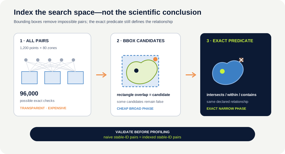
Every geometry has an axis-aligned minimum bounding rectangle described by minx, miny, maxx and maxy. Testing whether two rectangles overlap is much cheaper than evaluating the full relationship between complex polygon boundaries.

A bounding-box overlap means only:

These geometries are close enough in coordinate space to deserve an exact test.

It does not prove that the geometries intersect. A point can lie inside the bounding box of a crescent or ring polygon while remaining outside the polygon itself. Two complex polygons can have overlapping boxes but disjoint interiors.

This creates two stages:

1. Broad phase: retrieve geometries whose bounding boxes could match.
2. Narrow phase: apply the exact predicate—such as intersects, within or contains—to those candidates.

The broad phase should remove impossible pairs. The narrow phase preserves the scientific relationship.

4. A spatial index organises bounding boxes for search

A spatial index stores geometry bounding boxes in a search structure. GeoPandas uses Shapely's STRtree implementation for its spatial-index interface. STR means sort-tile-recursive: bounding boxes are packed into a tree so a query can discard large regions without visiting every stored geometry.

You do not need to implement the tree. You do need a correct mental model:

• the tree indexes bounding boxes, not ecological meaning;
• source geometries are not changed;
• returned integers are positional indices into the input collections;
• an unqualified query can include false-positive candidates;
• adding predicate= applies the exact relationship after the bounding-box filter;
• result order is not a scientific ordering and may differ between environments.

GeoPandas exposes the index through gdf.sindex. Inspect gdf.sindex.valid_query_predicates when designing a workflow. High-level operations including sjoin(), overlay() and clip() already use spatial indexing where appropriate. Building a second manual index around them does not automatically improve performance.

Check your understandingWhat does an overlapping spatial-index bounding box establish?

Choose one answer

Only that the pair is a candidate requiring the declared exact predicateThat the two geometries definitely intersectThat both geometries have the same CRS

Check answer

5. Generate a controlled performance scene

The following cell creates synthetic projected geometries near plausible EPSG:3301 coordinate magnitudes. They are deliberately regular so you can understand the workload. They do not describe a real site.

import geopandas as gpd
from shapely.geometry import Point

x0, y0 = 500_000, 6_450_000
plot_points = [Point(x0 + 10*x, y0 + 10*y)
               for y in range(30) for x in range(40)]
zone_centres = [Point(x0 + 40*x, y0 + 40*y)
                for y in range(8) for x in range(10)]
plots = gpd.GeoDataFrame(
    {"plot_id": [f"P{i:04d}" for i in range(len(plot_points))]},
    geometry=plot_points, crs="EPSG:3301")
zones = gpd.GeoDataFrame(
    {"zone_id": [f"Z{i:03d}" for i in range(len(zone_centres))]},
    geometry=gpd.GeoSeries(zone_centres, crs=plots.crs).buffer(18))

This produces 1,200 points and 80 rounded zone polygons. The naive search space therefore contains 96,000 possible pairs. The circles' rectangular bounds also create some candidate points that are inside a bounding box but outside the circular polygon, making the two stages observable.

Before continuing, audit row count, CRS, total bounds, geometry types, empty geometries and validity. A performance test on malformed or mismatched data is not an analytical success.

6. Worked example — compare equivalent match sets

Before running, predict which count must be equal for the two methods and which count may be larger. Do not predict an exact speed ratio.

from time import perf_counter

started = perf_counter()
naive = {(p.plot_id, z.zone_id) for p in plots.itertuples()
         for z in zones.itertuples() if p.geometry.intersects(z.geometry)}
naive_s = perf_counter() - started

started = perf_counter()
joined = plots.sjoin(zones[["zone_id", "geometry"]],
                     how="left", predicate="intersects")
join_s = perf_counter() - started
matched = joined.dropna(subset=["index_right"])
indexed = set(matched[["plot_id", "zone_id"]].itertuples(index=False, name=None))
unmatched = joined.loc[joined["index_right"].isna(), "plot_id"].nunique()
one_to_many = int((joined["plot_id"].value_counts() > 1).sum())

print("same matches:", naive == indexed)
print("rows/matches/unmatched/one-to-many:", len(joined), len(indexed), unmatched, one_to_many)
print("seconds:", {"naive": naive_s, "spatial_join": join_s})

Code walkthrough

1. perf_counter records elapsed time around two declared operations.
2. The nested comprehension visits every plot–zone pair and applies intersects directly.
3. Stable plot_id–zone_id pairs make correctness independent of output order.
4. sjoin(..., how="left", predicate="intersects") uses GeoPandas' indexed join while retaining unmatched plots.
5. matched separates rows with an actual right-side geometry before building the second stable-ID set.
6. unmatched counts unique left-side plots without a match.
7. one_to_many reveals plots represented by more than one joined row.
8. Row, matched, unmatched and repeated-ID evidence tests relational equivalence—not only set equality.
9. naive == indexed remains the decisive correctness check for matched pairs.
10. The timing dictionary reports one controlled run without implying universal performance.

If same matches is false, stop. Do not interpret the faster timing until you have found the difference in predicate, CRS, missing geometry, identifier mapping or result construction.

7. Measure the filter, not only the final answer

Run the spatial-index query once without a predicate:

candidates = zones.sindex.query(plots.geometry)
exact = zones.sindex.query(plots.geometry, predicate="intersects")
print("all possible pairs:", len(plots) * len(zones))
print("bbox candidates:", candidates.shape[1])
print("exact matches:", exact.shape[1])

The difference between all possible pairs and bounding-box candidates shows how much work the tree can avoid. The difference between bounding-box candidates and exact matches shows why the predicate stage remains necessary.

Index effectiveness depends on spatial arrangement. If every geometry's bounding box overlaps every other geometry, the index cannot discard much. A widely dispersed dataset with compact features may benefit more. A MultiPolygon whose distant parts share one large bounding box can also produce many unhelpful candidates.

8. Timing is evidence with conditions

One elapsed time is not a benchmark. First runs may include object creation, index construction, file-system cache effects or library initialisation. Very short operations can be dominated by measurement noise.

A defensible beginner profile records:

• Python, GeoPandas, Shapely and operating-system versions;
• input feature counts and geometry types;
• total possible, bounding-box candidate and exact-match counts;
• predicate and CRS;
• whether index construction is included;
• multiple repetitions after one warm-up;
• median or a small range, not only the fastest result;
• confirmation that stable match-ID sets are equal.

Use timeit for more controlled repetition after you understand which operation is timed. Do not optimise display, file reading and geometry comparison in one combined cell and then claim the spatial index caused the whole difference.

Speed is not the only resource constraint. A left spatial join materialises rows, attributes and geometry references; one-to-many relationships can make the output much larger than either input. A lower-level index query may use less intermediate tabular memory when only index pairs are required, while sjoin() provides clearer relational output for auditing. Record peak or approximate memory when scale makes it material, select only needed columns, and never discard unmatched or repeated rows merely to reduce memory.

Check your understandingWhich result must be checked before interpreting indexed and naive runtimes?

Choose one answer

The stable identifier-pair sets are equal under the same predicateThe indexed result appears first in the notebookThe two methods return rows in exactly the same order

Check answer

9. Common mistakes and recovery

Treating candidates as matches

Why it happens: the index returns pairs and the word “query” sounds definitive. Recognition: counts change when an exact predicate is added. Fix: use the bounding-box result for diagnosis only; apply the declared exact predicate before constructing the scientific relationship.

Comparing row order

Why it happens: two displayed tables appear different. Recognition: the same identifier pairs occur in another order. Fix: compare sets or sorted stable-ID pairs; index traversal order is not scientific evidence.

Timing unequal work

Why it happens: one method includes file reading or tree construction and the other does not. Recognition: cell contents and timed boundaries differ. Fix: define the operation, place timers around equivalent work and state what is included.

Reporting one speed-up as universal

Why it happens: a dramatic ratio looks informative. Recognition: the claim omits dataset size, geometry complexity, hardware or repetitions. Fix: report conditional evidence and explain why other datasets can behave differently.

Optimising before checking correctness

Why it happens: runtime is immediately visible, while a missing boundary case is subtle. Recognition: no stable-ID equivalence assertion exists. Fix: maintain a small trusted reference case and verify equality before profiling.

10. Guided practice — profile scale and spatial arrangement

Create a profiling table for three synthetic scenes:

1. small: 120 points and 20 zones;
2. medium: the 1,200-point, 80-zone scene above;
3. dense-overlap: reuse the medium scene but enlarge zone buffers so more bounding boxes overlap.

For each scene:

1. record feature counts and n × m possible pairs;
2. run a warm-up indexed query;
3. run the naive and indexed exact predicate at least three times;
4. compare stable identifier-pair sets after every run;
5. record bounding-box candidates and exact matches;
6. calculate candidate fraction as candidates divided by all possible pairs;
7. report median elapsed time for each method;
8. plot elapsed time against possible-pair count;
9. explain why the dense-overlap index filters less effectively;
10. state whether the evidence justifies a performance conclusion.

Required QA evidence

Your profile must show environment versions, CRS, feature and pair counts, candidate and match counts, repetitions, timed boundaries and an explicit equivalence result. Label all generated geometries as synthetic.

11. Independent challenge — design a trustworthy performance experiment

Design one additional experiment that changes only one property: number of points, number of polygons, polygon complexity or spatial clustering.

Before running it:

• state the hypothesis;
• identify the independent variable;
• identify what remains controlled;
• define the exact predicate and correct-result criterion;
• predict how candidate fraction may change.

Then run both methods, retain stable match pairs, use repeated timings and interpret the result. If the result contradicts your prediction, investigate rather than removing it. Possible explanations include index-build cost, nearly universal bounding-box overlap, measurement noise or Python-loop overhead.

Scientific interpretation

An indexed result can establish the same declared geometric relationship with fewer candidate comparisons. It does not improve positional accuracy, boundary provenance or ecological relevance. Faster containment of a plot within an outdated management polygon remains a fast answer to the wrong scientific representation.

12. Reflection, submission and portfolio artifact

Answer in your private notes:

1. Why is a bounding-box hit not an exact spatial match?
2. What must be equal before two implementations can be compared for speed?
3. When might a spatial index provide little benefit?
4. Why should timing conditions be recorded with the result?
5. Which high-level GeoPandas operations already use spatial indexing?

Submission

• Notebook: the continuing pipeline notebook with scene generation, naive and indexed implementations, candidate analysis and repeated profiling.
• File: spatial_index_profile.ipynb plus a CSV containing the profiling table.
• Screenshot: one labelled chart comparing workload and elapsed time across the three guided scenes.
• Written answer: 250–330 words explaining two-stage querying, equivalence evidence, timing limitations and the experiment outcome.

Portfolio artifact

Artifact 2.8 — Spatial performance benchmark and equivalence audit

This artifact demonstrates that you can improve a geospatial workflow without changing its scientific relationship. Add the equivalence assertion, candidate-efficiency table and conditional performance interpretation to the vector-processing stage of the UAV and Satellite Analysis Pipeline.