Geometry with Shapely

1. Make geometry express the scientific design

Learning outcome

By the end of this lesson, you will be able to distinguish geometry types, predicates, constructive operations and set operations; use Shapely geometry through GeoPandas; create metre-based plot-neighbourhood buffers; inspect validity and multipart results; and decide whether a computationally valid operation represents a defensible ecological support. You will add a documented geometry-decision record to the Module 2 pipeline.

Prerequisites: Complete Lesson 2.5. You should be able to audit a GeoDataFrame, identify its active geometry and CRS, and transform a copy to an appropriate projected CRS. Allow 90–120 minutes.

Why this matters

Geometry operations can transform an analysis more profoundly than a statistical formula. A point becomes a polygon when buffered. Two site boundaries become a smaller shared area when intersected. Several polygons become one geometry when united. Each result looks precise, but the precision belongs to the computation—not automatically to the ecological meaning.

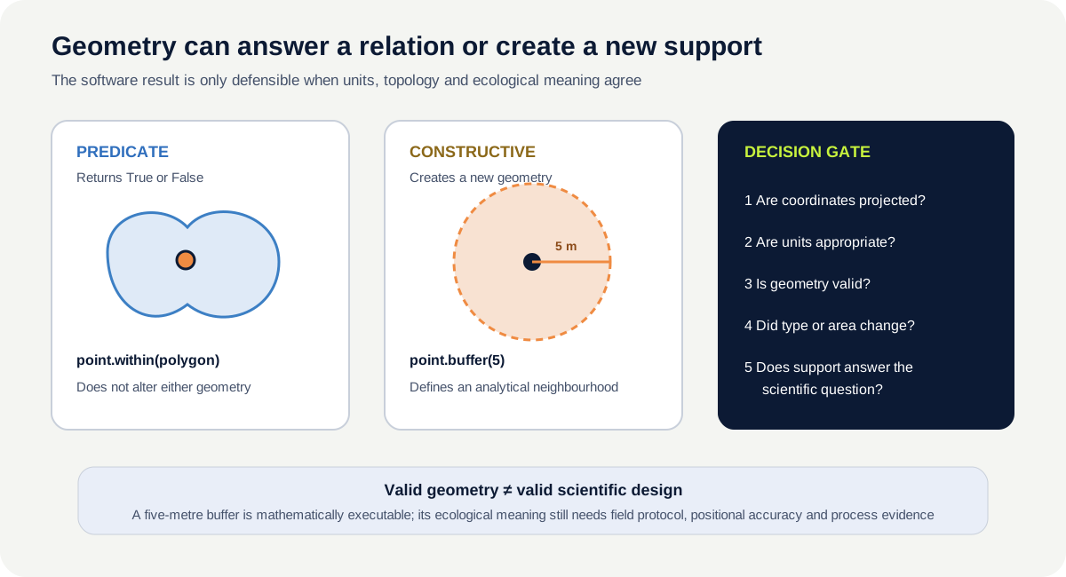
If a five-metre buffer is created around a field coordinate, what does the circle represent? The measured quadrat? GPS uncertainty? A vegetation neighbourhood? A raster-extraction window? These are different scientific claims, even though the code is identical.

Scientific standard: A computationally valid geometry operation may still be scientifically meaningless.

Scientific context

You are continuing with the synthetic vector training pack. The point coordinates were designed for instruction and have no survey accuracy. In a real Baltic coastal-meadow project, buffer size would need evidence from the sampling protocol, positional accuracy, ecological process and intended remote-sensing comparison.

In this lesson, a five-metre buffer is an analytical scenario, not a claim that any published plot sampled a five-metre radius. You will calculate it, audit it and then judge what additional evidence would be needed before scientific use.

Learner action

Add ## Lesson 2.6 — Geometry with Shapely to the pipeline notebook. Write one sentence completing this prompt: “A buffer around a field point represents ___ only if ___.” Keep the sentence visible while you work.

2. Geometry types represent different spatial ideas

Shapely models planar geometry. GeoPandas stores Shapely objects in a geometry column and applies operations across them.

• Point: a coordinate location with no area. It may represent a plot centre, instrument position or observation location.
• LineString: an ordered path with length but no area. It may represent a transect, shoreline segment or flight path.
• Polygon: an enclosed area with exterior and optional interior rings. It may represent a site boundary, management zone or explicit sampling footprint.

Geometry type is not a statement of measurement accuracy. A high-precision point can still represent a broad observation support. A polygon can have detailed vertices and still be an approximate management boundary.

Multipart geometry stores several parts as one feature: MultiPoint, MultiLineString or MultiPolygon. A site consisting of separated meadow patches may be a valid MultiPolygon. Do not explode it into separate features until you decide whether the parts share one identity or should become separate analytical units.

3. Predicates ask a question without changing geometry

A predicate evaluates a spatial relationship and returns True or False.

Examples include:

• point.within(polygon) — is every point of the first geometry inside the second geometry’s interior?
• polygon.contains(point) — the directional inverse for an interior point;
• geometry.intersects(other) — do the geometries share any spatial portion, including a boundary point?
• geometry.touches(other) — do they meet at boundaries without interior overlap?

Direction matters. “Point within zone” and “zone contains point” describe the same interior case from opposite arguments, but code and join orientation must match the question.

Boundary behaviour also matters. A point exactly on a polygon boundary is not within the polygon under the usual topological definition, but it intersects the polygon. Lesson 2.7 uses this difference to expose ambiguous assignments.

Check your understandingA point lies exactly on a polygon boundary. Which statement is correct?

Choose one answer

It intersects the polygon but is not within its interior under the usual topological definitionIt is always within and never touches the polygonThe result depends only on the point's attribute table

Check answer

4. Constructive operations create a new geometry

A constructive operation returns a geometry derived from an input.

Buffer

geometry.buffer(distance) creates a polygonal neighbourhood. For a point, positive distance produces an approximation to a circle. The distance uses coordinate units. A value of 5 means five metres only when the layer uses a suitable projected CRS with metre units.

Buffer design also includes resolution and, for lines, cap and join styles. Defaults are implementation choices, not ecological decisions. Record parameters when they affect area or shape.

Centroid

geometry.centroid returns a geometric centre of mass. For a concave polygon or MultiPolygon, the centroid can lie outside the represented area. A centroid is not automatically an observed location, accessible sampling point or ecological centre. If an interior label point is needed, a representative-point method may be more suitable—but it still does not create a measured coordinate.

Distance

geometry.distance(other) returns the minimum planar separation between geometries. It does not follow a path, terrain surface or coastline. Distance equals zero for intersecting geometries. Use projected units and define which spatial supports are being compared.

5. Set operations describe shared and combined space

Set-theoretic operations create geometry from the spatial relationship between inputs:

• intersection: the space shared by A and B;
• union: all space covered by A or B, with internal shared boundaries removed where appropriate;
• difference: the part of A not covered by B;
• symmetric difference: parts covered by one input but not both.

The output type can differ from the input type. Two polygons that touch only along an edge have a line-like intersection; polygons touching at one corner have a point-like intersection. Code that assumes every intersection is a polygon can silently discard meaningful boundary cases or fail later.

An operation is planar in GeoPandas and Shapely: z-values do not provide three-dimensional surface analysis. The CRS and chosen projection govern the coordinate plane.

6. Validity is a topological property, not a quality certificate

For polygons, validity asks whether rings and interiors satisfy topology rules. A bow-tie self-intersection is a common invalid polygon. Use both a Boolean check and the reason:

Valid geometry ≠ valid scientific design. A polygon can satisfy every topology rule while representing the wrong boundary, date, spatial support or ecological concept.

invalid = ~zones.geometry.is_valid
print(zones.loc[invalid, "zone_id"])
print(zones.loc[invalid].geometry.is_valid_reason())

Missing, empty and invalid geometries are different conditions. Report them separately.

Repair tools such as make_valid() can produce a MultiPolygon, GeometryCollection, line or empty result depending on the defect and method. Therefore:

1. preserve the original geometry;
2. record the validity reason;
3. repair only with a stated rule;
4. compare geometry type, part count, feature count and area before and after;
5. review the result against domain evidence.

Do not apply a universal repair to every feature simply because the method returns without an error.

Check your understandingWhat does a valid polygon establish?

Choose one answer

Its topology is well formed; scientific meaning, positional accuracy and appropriate support still need evidenceIts boundary is ecologically correct and currentIts centroid must lie inside and represent a sampled location

Check answer

7. Worked example — define and audit plot neighbourhoods

Before running, predict the output geometry type and the approximate area of a circle with radius five metres. Why might the computed area differ slightly from π × 5²?

from pathlib import Path
import geopandas as gpd

path = Path("data/training/vector_foundations/training_field_plots.geojson")
plots = gpd.read_file(path).to_crs("EPSG:3301")
radius_m = 5
neighbourhoods = plots[["plot_id", "geometry"]].copy()
neighbourhoods["geometry"] = plots.geometry.buffer(radius_m)
neighbourhoods["area_m2"] = neighbourhoods.geometry.area

print(neighbourhoods.geom_type.value_counts())
print(neighbourhoods["area_m2"].round(2))
print("all valid:", bool(neighbourhoods.geometry.is_valid.all()))

The result should contain polygon neighbourhoods with broadly similar areas close to the theoretical circle area. Small differences reflect polygonal approximation and library parameters. Equal computed areas do not establish equal ecological relevance or positional accuracy.

Code walkthrough

1. Path identifies the immutable training input.
2. GeoPandas is imported as gpd.
3. The points are read and transformed to EPSG:3301 so the operation uses metre-based projected coordinates.
4. radius_m gives the number a unit and makes the design parameter visible.
5. Only stable identity and geometry are copied into the derivative.
6. buffer(radius_m) creates one polygonal neighbourhood per point.
7. Replacing the derivative’s active geometry does not alter the raw plots object.
8. .area calculates planar polygon area in square metres for this target CRS.
9. The geometry-type count checks that the constructive operation produced the expected family.
10. Rounded areas support reporting without changing stored geometry.
11. The validity check confirms topological form, not scientific design.

The outlying training point also receives a valid five-metre buffer. This is deliberate evidence that geometric success does not enforce study membership.

8. Audit a geometry operation as a before-and-after transformation

Every geometry-changing step should preserve a decision record:

Evidence	Before	After
source object	training points	neighbourhood derivative
CRS and units	EPSG:3301, metres	EPSG:3301, metres
feature count	expected point count	expected neighbourhood count
stable IDs	unique plot_id	same IDs
geometry type	Point	Polygon
missing/empty/invalid	reported	reported again
area or length	not applicable	distribution and expected range
parameter	none	radius and buffer options
scientific rationale	point location	proposed analytical support

Compare, do not merely record. A lost ID, changed feature count, empty output or surprising area is a diagnostic signal.

Check your understandingWhen can buffer(5) be interpreted as a five-metre ecological neighbourhood?

Choose one answer

When the CRS uses suitable metre units and independent scientific evidence justifies that supportWhenever the layer appears on a web mapWhenever every output polygon is valid

Check answer

9. Common mistakes and recovery

Buffering longitude and latitude

Why it happens: the geographic layer plots correctly. Recognition: a buffer distance is interpreted in degrees or triggers a warning. Fix: transform a copy to a justified projected CRS and verify its units before buffering.

Calling the buffer a sampled area

Why it happens: the circle surrounds the field point. Recognition: the interpretation claims field support without a sampling-protocol reference. Fix: label it as an analytical neighbourhood and justify support from independent evidence.

Assuming the centroid lies inside

Why it happens: the word “centre” suggests membership. Recognition: centroids fall in a hole, water area or outside a concave boundary. Fix: inspect the geometry and choose a method appropriate to the purpose; never present a derived point as observed.

Repairing every polygon automatically

Why it happens: validity errors block later operations. Recognition: type or area changes without review. Fix: preserve the source, record the defect, apply a stated repair and audit the changed geometry.

Ignoring multipart outputs

Why it happens: maps draw all parts as one feature. Recognition: code assumes .exterior, one centroid or one area component. Fix: inspect geometry type and part structure, then decide whether feature identity or separate parts should drive analysis.

10. Guided practice — compare three geometry questions

Use the transformed training points and study-area polygon.

Question A — membership predicate

For each point, evaluate whether it is within the study area and whether it intersects the study area. Identify the interior, boundary and outside cases. Explain the boundary rule in words.

Question B — neighbourhood support

Create 1 m, 5 m and 10 m buffers around each point. For every radius:

1. record CRS and units;
2. calculate theoretical circle area;
3. compare computed area and relative difference;
4. report validity, empty count and geometry type;
5. intersect neighbourhoods with the study area;
6. calculate the fraction of each neighbourhood retained;
7. identify plots whose analytical support extends outside the site.

Question C — combined site geometry

Union the two management-zone polygons. Compare feature count, geometry type and total area before and after. Then intersect the management and vegetation zones. Explain why the intersection creates new analytical units rather than simply attaching attributes.

Required QA evidence

Provide a table containing operation, input CRS, parameter, input type/count, output type/count, missing, empty, invalid, area change and scientific purpose. Include a diagnostic plot that distinguishes original geometry from derived geometry.

11. Independent challenge — defend or reject a support rule

A collaborator proposes extracting UAV reflectance from a 10 m buffer around every field point because larger neighbourhoods “average noise.” Write a technical response and test the geometry.

Your response must:

• distinguish field support, positional uncertainty and smoothing;
• calculate the 10 m neighbourhood area relative to a 1 m² quadrat;
• identify overlap with site boundaries and neighbouring buffers;
• state which acquisition and georegistration evidence is missing;
• propose at least two alternative support rules;
• define a sensitivity analysis across plausible radii;
• state when the proposed buffer should be rejected.

Do not choose the radius producing the strongest ecological relationship. Define the rationale before comparing results.

Scientific interpretation

The geometry analysis can show exactly which area a rule creates, where it crosses boundaries and how sensitive it is to radius. It cannot prove that the area represents vegetation sampled in the field, sensor response or a meaningful ecological neighbourhood. Those interpretations require field and sensor evidence.

12. Reflection, submission and portfolio artifact

Answer in your private notes:

1. How does a predicate differ from a constructive operation?
2. Why can a valid polygon still be scientifically unsuitable?
3. Under what conditions is distance() expressed in metres?
4. Why can geometry repair change the data model?
5. What evidence would justify a plot-neighbourhood radius?

Submission

• Notebook: the continuing pipeline notebook with the worked buffer, three-question guided practice and independent support review.
• File: plot_neighbourhoods.ipynb plus a GeoPackage layer containing the clearly labelled training derivatives.
• Screenshot: original points, three buffer radii and clipped support, with units and synthetic status visible.
• Written answer: 180–250 words defending one support rule and stating what it does not prove.

Portfolio artifact

Artifact 2.6 — Geometry-operation and plot-neighbourhood decision record

This artifact demonstrates that you can separate geometric execution from scientific justification. Add the parameter table, before-and-after audit and sensitivity design to the spatial-support stage of the UAV and Satellite Analysis Pipeline.