Scale, Resolution and Spatial Support

1. Ask what physical area produced each value

Learning outcome

By the end of this lesson, you will be able to distinguish spatial scale, grain, extent, raster resolution and spatial support. You will compare a one-square-metre field quadrat, a 5 cm UAV pixel and a 10 m Sentinel-2 pixel, identify mixed-pixel and scale-mismatch risks, and create a documented support-matching decision for the Baltic coastal-meadow workflow.

Prerequisites: Complete Lessons 2.1–2.2. You should understand vector and raster representations, CRS units and why a smaller coordinate or pixel number is not automatically better evidence. Allow 90–120 minutes.

Why this matters

Remote-sensing studies often place field values and image values in the same table, then model their relationship. The rows align, the code runs and the scatterplot looks convincing. Yet the observations may describe very different physical areas.

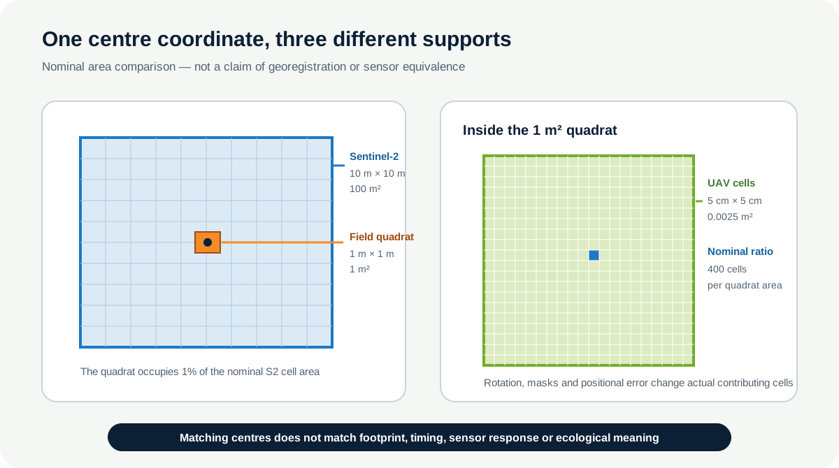
A biomass harvest from one square metre integrates plants within a quadrat. A 5 cm UAV pixel represents a much smaller ground cell, influenced by the sensor response, motion, illumination and georegistration. A 10 m Sentinel-2 pixel covers 100 square metres and may combine meadow vegetation, soil, water, litter and shadow. Matching their centres does not make their support equal.

Core spatial question: Do the measurements describe compatible physical areas, times and ecological processes?

Scientific context

The Module 1 field table provides ecological measurements for Baltic coastal-meadow quadrats but no published coordinates. In this instructional design exercise, assume that a future, separately governed coordinate table has been verified and that the field protocol defines a 1 m × 1 m quadrat. The 5 cm UAV and 10 m Sentinel-2 values are scale examples from the technical specification, not claims about files included in the Zenodo record.

Your objective is not to force these observations into one scale. It is to design and justify how they could be compared, then state the uncertainty that remains.

Learner action

Add ## Lesson 2.3 — Scale, resolution and spatial support to the continuing notebook. Write one ecological pattern you expect at centimetre scale and one that requires a larger landscape extent. This anchors the technical discussion in a scientific question.

2. Scale has several meanings

The word scale is used in different ways across cartography, ecology and remote sensing. Avoid using it alone when a more precise term is available.

• Grain is the size of the smallest spatial unit represented or sampled in an analysis. For a regular image, pixel size is an important part of grain.
• Extent is the total area covered by the dataset or analysis.
• Map scale describes the relationship between distance on a map and distance on the ground. It matters for visualisation and generalisation but is not the same as raster pixel size.
• Process scale is the spatial range over which an ecological process operates—for example, plant-level stress, within-patch hydrology or landscape connectivity.

Fine grain and broad extent are independent ambitions. A UAV survey can offer centimetre-scale pixels over a limited site. A satellite mission can repeatedly cover a much wider region at coarser spatial resolution. Neither is universally superior; each provides evidence for different questions.

3. Resolution is not a synonym for accuracy

For a raster, spatial resolution is often communicated through ground pixel size. Sentinel-2 has bands delivered at 10 m, 20 m and 60 m spatial resolutions. The number does not describe every aspect of the observation.

Keep these properties separate:

• pixel size: the dimensions of a grid cell in ground units;
• effective resolving ability: how well neighbouring targets can actually be distinguished, influenced by optics, sampling and processing;
• positional accuracy: how close the represented location is to its true location;
• radiometric quality: how reliably the sensor records differences in signal;
• spectral resolution: the number, width and placement of spectral bands;
• temporal resolution: how frequently comparable observations are available.

Upsampling a 10 m image to 5 cm creates more cells. It does not create the missing fine-scale observations. Interpolation estimates values on a denser grid from existing information.

Check your understandingA 5 cm UAV pixel is smaller than a 10 m Sentinel-2 pixel. What follows?

Choose one answer

It samples a finer grid, but accuracy and ecological relevance still require separate evidenceIt is automatically more accurate for every variableIt can be compared directly with one square-metre biomass without aggregation

Check answer

4. Spatial support belongs to the measurement

Spatial support is the physical area and geometry over which one reported value is observed, integrated or aggregated. Support is not merely where the centre point lies.

Consider three values:

1. A field biomass value from a 1 m² quadrat integrates material collected according to a field protocol over that footprint.
2. One 5 cm UAV reflectance pixel represents a nominal 0.0025 m² grid cell, but the recorded signal can be influenced by the sensor point-spread response and processing.
3. One 10 m Sentinel-2 pixel represents a nominal 100 m² grid cell for a 10 m band.

Even if all three share a centre coordinate, they observe different neighbourhoods. Extracting a single UAV pixel at the quadrat centre discards most of the sampled footprint. Extracting one satellite pixel for a quadrat may attach a 100 m² mixed signal to a 1 m² field measurement.

Check your understandingWhat does spatial support describe?

Choose one answer

The physical area and geometry over which one value is observed or aggregatedOnly the pixel width written in a filenameThe total number of rows in a table

Check answer

Temporal support belongs to the observation too

Temporal support is the instant or interval over which a reported value is observed, integrated or summarised. A field measurement taken during one morning, a UAV mosaic assembled from a 25-minute flight and a monthly satellite composite do not share the same temporal support even if they use the same date label.

Before combining observations, build a support matrix:

Observation	Spatial support	Temporal support	Measurement process
biomass quadrat	documented 1 m² footprint	harvest date and sampling interval	clipped, dried and weighed vegetation under the field protocol
UAV reflectance	pixel response and extraction footprint	flight start/end time and mosaic inputs	calibrated camera observations processed into an orthomosaic
Sentinel-2 reflectance	band-specific pixel support	acquisition instant; or stated composite interval	satellite sensor response and product processing

The third column prevents “same location” from becoming “same observation.” The measurement-process column prevents spatial and temporal alignment from being mistaken for equivalence of ecological meaning.

5. Worked example — compare nominal support areas

Predict the three reported areas and two ratios before running. Pay attention to the difference between metres and square metres.

supports = {
    "field_quadrat": {"width_m": 1.0, "height_m": 1.0},
    "uav_pixel": {"width_m": 0.05, "height_m": 0.05},
    "sentinel2_pixel": {"width_m": 10.0, "height_m": 10.0},
}

areas = {
    name: item["width_m"] * item["height_m"]
    for name, item in supports.items()
}
for name, area_m2 in areas.items():
    print(name, area_m2, "m²")

print("UAV cells per quadrat area:", areas["field_quadrat"] / areas["uav_pixel"])
print("Quadrat share of S2 cell:", areas["field_quadrat"] / areas["sentinel2_pixel"])

Expected numerical relationships:

• the quadrat covers 1.0 m²;
• a 5 cm × 5 cm UAV cell covers 0.0025 m²;
• a 10 m × 10 m Sentinel-2 cell covers 100.0 m²;
• 400 nominal UAV cells equal the quadrat area;
• the quadrat area is 0.01, or one percent, of one 10 m satellite cell.

Code walkthrough

1. supports stores widths and heights with units visible in the key names.
2. The quadrat and two pixels are described using the same structure so the calculation is consistent.
3. The dictionary comprehension multiplies linear dimensions to obtain area.
4. area_m2 names the result as square metres, preventing a unit from becoming implicit.
5. The first ratio divides quadrat area by UAV-cell area.
6. The result 400 is an area equivalence, not a guarantee that exactly 400 usable pixels fall inside a georeferenced quadrat polygon.
7. The second ratio shows that one quadrat occupies only one percent of a 10 m cell in nominal area.

These ratios reveal the problem; they do not solve it. Rotation, boundary placement, georegistration, sensor response and missing pixels affect the actual contributing cells.

6. Mixed pixels are ecological mixtures

A mixed pixel receives signal from more than one relevant surface or state. In a coastal meadow, a satellite pixel might combine vegetation communities, bare sediment, standing water and shadows. The resulting reflectance is not necessarily a simple ecological average. Different materials interact with illumination, canopy structure and the atmosphere in different ways.

Mixture depends on the target question. A pixel containing two plant species may be mixed for species mapping but acceptably homogeneous for a broad vegetated-versus-water classification. “Mixed” must therefore be defined relative to the phenomenon and decision.

At boundaries, small positional errors change mixture substantially. A 2 m shift may be modest within a 10 m homogeneous meadow pixel but decisive for a 5 cm UAV extraction or a narrow vegetation strip.

7. Matching support requires an explicit rule

Common support-matching strategies include:

• point extraction: use the raster cell containing a verified point;
• footprint mean or median: summarise raster cells within the documented quadrat polygon;
• buffered extraction: summarise a neighbourhood justified by positional uncertainty or ecological influence;
• aggregation to a common grid: combine finer cells into larger units using a documented statistic;
• stratified comparison: compare only spatially homogeneous regions or report components separately;
• hierarchical modelling: retain observations at their native supports and model the relationship explicitly.

No method is automatically correct. A footprint mean may fit a quadrat-integrated field measurement, while a buffer may better represent coordinate uncertainty. A median is robust to extreme pixels but changes the estimand. The choice must be defined before looking for the strongest correlation.

Record at least:

Decision	Required evidence
target variable	ecological quantity and unit
field support	footprint, protocol and date
image support	pixel size, band/product, date and mask
alignment	CRS, transform and positional accuracy
extraction rule	point, footprint, buffer or aggregation
weighting	equal, area-weighted or quality-weighted
completeness	minimum valid coverage and missing-data rule
uncertainty	mismatch that the method cannot remove

8. Extent and sampling change what can be inferred

A 5 cm UAV product may reveal within-quadrat gaps, leaf clusters, flowers, shadows and fine drainage features, while missing broader landscape context. Sentinel-2 can support repeated site-to-region observation, while a 10 m pixel cannot isolate a single 1 m² quadrat.

Increasing extent can include more environmental gradients, but it also introduces new land covers, atmospheric conditions and management regimes. Increasing grain size smooths local variability. Decreasing grain size can expose noise and registration error. Study design must balance the scale of the process, the observation mechanism and the inference target.

9. An introduction to MAUP

The modifiable areal unit problem, or MAUP, is the observation that statistical results can change when the same underlying data are grouped into zones of different sizes or arrangements.

Imagine summarising UAV reflectance by:

• exact quadrat polygons;
• 1 m grid cells aligned differently;
• management zones;
• whole sites.

The means, variances and correlations can differ because aggregation changes which observations are combined. This does not make areal summaries invalid. It means the reporting unit is part of the method and must have a scientific rationale.

Choose zones before comparing preferred results. If several plausible zone definitions exist, use a sensitivity analysis and report how conclusions change.

Check your understandingWhy should an aggregation boundary be chosen before inspecting preferred results?

Choose one answer

Changing zones can change the statistic, so the choice needs an independent scientific rationaleAll boundaries produce identical summariesAggregation removes mixed pixels

Check answer

10. Common mistakes and recovery

Calling the smallest pixel the best dataset

Why it happens: finer images look detailed. Recognition: the argument mentions pixel size but not calibration, coverage, timing, accuracy or process scale. Fix: evaluate fitness for the ecological question across all relevant dimensions.

Comparing a quadrat to one centre pixel

Why it happens: point sampling is easy. Recognition: the extraction footprint does not match the field protocol. Fix: represent or reconstruct the quadrat support and justify the raster summary.

Upsampling to create detail

Why it happens: smaller output cells resemble higher resolution. Recognition: the output grid is finer but the input observation has not changed. Fix: state that resampling changes representation and preserve the native-resolution evidence.

Ignoring acquisition time

Why it happens: spatial overlap dominates the workflow. Recognition: field, UAV and satellite dates or phenological stages are absent from the support table. Fix: treat temporal support as part of comparability.

Selecting aggregation zones after seeing correlations

Why it happens: one configuration appears to “work better.” Recognition: no independent rationale or sensitivity analysis exists. Fix: predefine the main support and report alternatives transparently.

11. Guided practice — build a support-matching decision table

Create a table for field biomass, UAV reflectance and a Sentinel-2 10 m band.

1. Record the nominal footprint and area of each observation.
2. Record what the value physically represents; do not write only the filename.
3. Add acquisition date or required temporal tolerance.
4. List the main geolocation uncertainty.
5. State what ecological variation each support can resolve, mix or miss.
6. Propose a quadrat-to-UAV extraction rule.
7. Propose a quadrat-to-Sentinel validation design using multiple field observations or homogeneous reference areas.
8. Define the minimum valid-pixel coverage required for a summary.
9. State one mismatch that remains after the proposed processing.

Do not calculate an ecological correlation in this lesson. Your output is the design that must exist before a defensible comparison.

Required QA evidence

Include correct linear and area units, a diagram of the three supports, and a written aggregation rule. Explain why nominal area equivalence does not guarantee spatial alignment.

12. Independent challenge — test sensitivity to support

Design a small synthetic experiment using a 20 × 20 array representing centimetre-scale vegetation reflectance.

• Create a patchy surface with at least two zones and one missing region.
• Calculate summaries for four adjacent 10 × 10 blocks.
• Shift the block origin by a few cells and recalculate.
• Compare the means and rank order of the zones.
• Explain how this illustrates boundary sensitivity and introductory MAUP.

Keep the example clearly synthetic. Do not describe the array as measured UAV data. Your interpretation should focus on how support and zoning change summaries, not on vegetation conclusions.

Scientific interpretation

The support analysis can show whether observations are physically comparable enough for a proposed method and where aggregation choices affect results. It cannot guarantee that sensors measure the same ecological quantity, remove temporal mismatch or validate a proxy such as NDVI against biomass. Those questions require sensor knowledge, field design and independent validation.

13. Reflection, submission and portfolio artifact

Answer in your private notes:

1. What is the difference between pixel size and spatial support?
2. Why can a 5 cm UAV product be less useful than Sentinel-2 for some questions?
3. What does a mixed pixel mean relative to your target variable?
4. How could a positional error affect UAV and satellite extractions differently?
5. Which part of a support decision should be tested with sensitivity analysis?

Submission

• Notebook: the continuing pipeline notebook with area calculations, the support-matching table and synthetic sensitivity challenge.
• Screenshot: the three-support diagram or the completed decision table with units visible.
• Written answer: 180–240 words proposing a defensible comparison between one field measurement and imagery. State what each scale can observe, the extraction rule and the unresolved uncertainty.

Portfolio artifact

Artifact 2.3 — Spatial support decision

This artifact demonstrates that you can define the observation footprint before extracting pixels or fitting a model. It becomes the scientific design record used later for raster–vector integration, UAV analysis and satellite validation.

Keep the reviewed checkpoint in the continuing notebook and export it as spatial_support_decision.ipynb for submission.

Species-to-pixel bridge

The Academy field response belongs to a 1 m² quadrat; UAV and satellite values belong to sensor-dependent pixel footprints or plot aggregations. Fine resolution does not remove support mismatch. Use the leaf-to-landscape scale explainer.