Geospatial Formats and Metadata

1. Choose a format from the scientific and operational requirement

Learning outcome

By the end of this lesson, you will be able to choose an appropriate format for field points, large analytical vector data, analysis-ready rasters and multidimensional Earth Observation data. You will explain the tradeoffs among Shapefile, GeoPackage, GeoJSON, GeoParquet, GeoTIFF, Cloud Optimized GeoTIFF, NetCDF and Zarr, and define post-conversion checks that protect scientific meaning.

Prerequisites: Complete Lessons 2.1–2.3. You should understand spatial models, CRS, extent, grid structure and spatial support. Allow 90–120 minutes.

Why this matters

File format is not an administrative detail. It affects which field names survive, how missing values are represented, whether CRS and NoData metadata remain attached, how much data must be read, and which collaborators can open the result.

A technically successful conversion can still damage the evidence. A field name may be truncated, an integer may replace a nullable value, a raster mask may disappear, or a data cube may lose coordinate attributes. A professional workflow chooses a format deliberately and verifies the derivative before it is accepted.

Core spatial question: Which representation preserves the required scientific structure and supports the way the data will actually be accessed?

Scientific context

The Baltic coastal-meadow pipeline will eventually contain:

• verified field or control-point vectors edited locally;
• larger vector tables used mainly for analytical filtering and joins;
• UAV and satellite raster products accessed by geographic subset;
• time × band × y × x Earth Observation arrays;
• metadata, provenance and quality decisions connecting every derivative to its source.

No single format is best for all of these. Your task is to create a format decision register that can be reviewed before data are converted or published.

Learner action

Add ## Lesson 2.4 — Geospatial formats and metadata to the Module 2 notebook. List three formats you have encountered. For each, write what you know from evidence and what you currently assume. This separates familiarity from fitness.

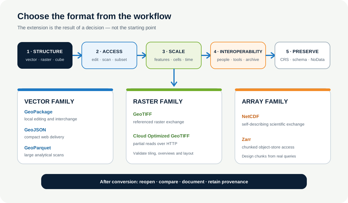
2. Evaluate formats with five questions

Use the same decision sequence for every asset:

1. Structure: Is the information tabular, vector, a two-dimensional raster or a multidimensional labelled array?
2. Access pattern: Will people edit it locally, scan selected columns, read geographic windows over HTTP, or analyse chunks across time?
3. Scale: How many features, pixels, bands and time steps exist, and how quickly will the data grow?
4. Interoperability: Which desktop GIS, Python libraries, databases, web clients and archives must use it?
5. Preservation: Which CRS, schema, geometry, NoData, units, attributes and provenance must survive?

These questions produce a conditional decision, not a universal ranking. A small GeoJSON file can be excellent for web exchange and poor for a national analytical archive. A GeoPackage can be excellent for local editing and inappropriate for massively parallel object-store access.

3. Vector formats serve different workflows

Shapefile — important legacy, weak default for new work

The ESRI Shapefile remains common and many systems read it. Its limitations matter:

• one logical layer is split across required and optional sidecar files;
• field names are restricted to ten characters in the DBF component;
• attribute types and missing-value handling are limited compared with modern tables;
• one file represents one geometry type;
• CRS information depends on a separate .prj file and may not carry all modern metadata cleanly;
• text encoding can depend on additional conventions or a .cpg file.

Calling Shapefile legacy does not mean every existing Shapefile should be rejected. Preserve source archives and support required clients. For new analytical products, choose a modern format unless compatibility requirements justify the constraints.

GeoPackage — strong local interchange and editing

GeoPackage is an OGC standard built on SQLite. One .gpkg file can contain multiple vector layers, attributes and other supported content, with modern field names and CRS definitions. It works well for compact project delivery, desktop GIS and governed local exchange.

It is not designed as a cloud object-store format for parallel scans. Concurrent multi-user editing and very large enterprise workloads may be better served by a spatial database.

Check your understandingWhich format is the strongest default for an editable multi-layer local vector project?

Choose one answer

GeoPackageA loose Shapefile componentA screenshot of the map

Check answer

GeoJSON — readable web exchange

GeoJSON represents feature collections and geometry in JSON. It is human-readable, widely supported by web clients and useful for small-to-moderate delivery. RFC 7946 defines positions in WGS 84 longitude and latitude order.

Text representation can be verbose for large datasets, and the format is not a substitute for a rich analytical schema or spatial index. Reprojection to web-delivery coordinates is a scientific operation: preserve an analysis-ready source and record the derivative.

GeoParquet — columnar analytical vectors

GeoParquet adds geospatial metadata and geometry encoding conventions to Apache Parquet. Columnar storage, compression and selective column reads can make it effective for large analytical vector tables and cloud workflows.

Support across tools is growing, but the receiving environment must be tested. Treat the version of the GeoParquet specification and geometry encoding as part of the contract. A performance-oriented format is only useful if collaborators can read it correctly.

4. Raster formats separate data model from access layout

GeoTIFF — a referenced raster asset

GeoTIFF stores raster cells with georeferencing information embedded through TIFF tags and related conventions. It is broadly supported and appropriate for many two-dimensional or multiband raster products. Important creation choices include data type, compression, tiling, block size, NoData or masks, band descriptions and overviews.

A .tif extension does not prove that georeferencing is complete or that the file is cloud optimised. Inspect the internal profile.

Cloud Optimized GeoTIFF — organised for partial remote reads

A Cloud Optimized GeoTIFF, or COG, is a GeoTIFF whose internal tiling, overview structure and file organisation support efficient HTTP range requests. A client can request the byte ranges needed for a geographic window or zoom level instead of downloading the entire raster.

COG does not create a new scientific raster model. The values, CRS, transform, bands and NoData semantics still require the same validation. A file should be validated against the COG layout requirements rather than called a COG because it is stored online.

Check your understandingWhat makes a Cloud Optimized GeoTIFF useful for remote access?

Choose one answer

Internal tiling, overviews and file organisation that support HTTP range requestsIt removes the need for CRS and NoData metadataIt converts every raster into a multidimensional data cube

Check answer

5. Multidimensional formats preserve labelled structure

Remote-sensing analysis often extends beyond band × y × x to time × band × y × x, with coordinate labels and attributes.

NetCDF

NetCDF is a long-established, self-describing format and data model for multidimensional scientific arrays. Variables can use named dimensions and carry attributes such as units and conventions. It is common in climate, ocean and atmospheric science and can be highly interoperable when communities follow conventions such as CF metadata.

A single NetCDF file can be convenient for exchange and archiving, but performance depends on variable layout, chunking and compression. “Self-describing” does not guarantee that every variable is documented well.

Zarr

Zarr stores chunked, compressed N-dimensional arrays with metadata, commonly across a directory-like hierarchy or object store. Independent chunks support parallel and subset access without reading one monolithic file.

Chunk shape is a design decision. Chunks optimised for reading one time slice may be inefficient for extracting a long pixel time series. Large numbers of very small objects can also create overhead. Record the Zarr specification version, chunking, compression and consolidation choices where applicable.

NetCDF and Zarr overlap in purpose but differ in storage and access characteristics. Choose from the real workflow, not from a slogan that one format is “modern.”

6. Metadata are part of the scientific product

At minimum, preserve or accompany each asset with:

• title and concise description;
• creator and contact or responsible organisation;
• source dataset and stable identifier;
• licence and access constraints;
• acquisition or observation time;
• processing history and software versions;
• CRS and spatial extent;
• geometry type or raster dimensions and bands;
• units and valid-value definitions;
• NoData, mask and quality-flag meaning;
• spatial and temporal support;
• known limitations;
• checksum for immutable deliveries.

Some metadata live inside the format. Other information belongs in a catalogue record, README, STAC item, data dictionary or provenance log. Embedded metadata can still be wrong. Validate it against the source and method.

Sidecar files

A sidecar is a separate file needed to interpret or support the main file. Shapefile uses several components. A raster may have an external mask, overview, world file or auxiliary metadata. Sidecars increase the risk that copying only the obvious file will create an incomplete dataset.

Use an inventory or manifest to identify all required components. Package or migrate them deliberately rather than relying on folder memory.

7. Worked example — record a format decision

Before running, predict which choice supports partial raster reads and which supports chunked multidimensional arrays.

decisions = [
    ("editable field points", "GeoPackage", "single local multi-layer container"),
    ("large analytical vectors", "GeoParquet", "columnar selective reads"),
    ("analysis-ready raster", "COG", "windowed HTTP range access"),
    ("EO data cube", "Zarr", "chunked N-dimensional access"),
]

for product, selected_format, reason in decisions:
    print(f"{product}: {selected_format}")
    print(f"  reason: {reason}")

Code walkthrough

1. decisions is a list because the register contains several product decisions in a deliberate order.
2. Each tuple keeps the product, selected format and primary reason together.
3. The first decision prioritises local editing and compact interchange.
4. The second prioritises analytical column access for large vectors.
5. The third prioritises partial remote raster reads.
6. The fourth prioritises chunked multidimensional access.
7. The loop applies the same reporting structure to every decision.
8. The first print line shows the choice; the second exposes the reason instead of presenting an unexplained extension.

This is a starting register, not a complete decision. Add scale, receiving tools, rejected alternative, limitation and post-conversion validation before approving a production format.

8. Verify every conversion

A conversion is complete only after the derivative has been reopened and compared with the source.

Use checks appropriate to the data model:

Vector conversion checks

• feature count and stable identifiers;
• geometry type, emptiness and validity;
• CRS and bounds;
• field names, types, null counts and categorical values;
• text encoding and representative strings;
• layer names and spatial index where expected.

Raster conversion checks

• CRS, transform, bounds, resolution and dimensions;
• band count, order, names and units;
• data type, scale/offset and valid range;
• NoData value, internal mask and missing-cell count;
• compression, tiling, block size and overviews;
• representative statistics or checksums according to the transformation.

Multidimensional conversion checks

• variable and dimension names;
• coordinate values and ordering;
• CRS or grid-mapping information;
• attributes and units;
• chunk shape, compression and fill values;
• equality or tolerance checks on representative subsets.

Keep the source. If a conversion changes the data intentionally—for example, reprojecting or changing data type—record the method, parameters and expected numerical consequences.

Check your understandingWhen is a format conversion complete?

Choose one answer

After reopening the derivative and verifying schema, CRS, counts, NoData and provenanceAs soon as the output path existsWhen the file extension looks modern

Check answer

9. Performance and file size are access questions

Compression reduces storage and transfer but costs computation. Chunking and tiling determine which parts can be read efficiently. Overviews accelerate low-resolution raster display. Columnar storage avoids loading unused attributes. Spatial indexes reduce candidate searches.

Do not optimise from file size alone. Ask how people will read the data:

• whole file once;
• repeated map windows;
• a few columns across millions of features;
• one pixel through hundreds of dates;
• complete time slices over a region;
• local editing by one person;
• concurrent queries by many users.

Benchmark representative operations and preserve the measurement conditions. One laptop timing is not a universal performance claim.

10. Common mistakes and recovery

Choosing Shapefile by habit

Why it happens: it opens almost everywhere. Recognition: long field names, nulls or metadata are lost without a documented requirement. Fix: preserve required legacy delivery when necessary, but use a modern analytical master and validate the export.

Calling any online TIFF a COG

Why it happens: “cloud” describes location in everyday language. Recognition: internal tiling, overviews and range-read layout were never validated. Fix: inspect and validate the asset against COG requirements.

Choosing Zarr without designing chunks

Why it happens: the format is associated with scale. Recognition: common queries touch hundreds of tiny objects or load unnecessary dimensions. Fix: define access patterns and test chunk layouts on representative operations.

Deleting the source after a successful write

Why it happens: the derivative appears equivalent. Recognition: no comparison report or recovery path exists. Fix: retain the immutable source according to governance policy until preservation and QA are independently confirmed.

Treating metadata as documentation added later

Why it happens: producing the data feels like the main work. Recognition: units, masks, processing history or licence cannot be reconstructed. Fix: create metadata during acquisition and processing, and test required fields before release.

11. Guided practice — complete a format selection matrix

Create one row for each product:

1. verified field points edited in QGIS and Python;
2. a 20-million-feature vector archive used for analytical filtering;
3. a 60 GB orthomosaic accessed by geographic windows over HTTP;
4. a ten-year time × band × y × x Earth Observation cube.

For every row, record:

• data structure and estimated scale;
• primary and secondary access patterns;
• required receiving tools;
• selected working format;
• selected delivery or archive format if different;
• one rejected alternative and why;
• required internal and external metadata;
• post-conversion QA;
• one limitation that remains.

Do not delete source data. The objective is a defensible decision, not a conversion race.

Required QA evidence

Your matrix must explicitly distinguish GeoTIFF from COG and NetCDF from Zarr. Include a preservation test for CRS, schema or grid, missingness and provenance for every product.

12. Independent challenge — design a two-audience delivery

The research group must deliver a coastal-meadow vector layer to:

• local environmental staff who edit the layer in desktop GIS;
• data scientists who scan selected columns across a national archive in Python.

Design a two-format delivery rather than forcing one file to serve both audiences. Specify:

• authoritative source and versioning approach;
• desktop delivery format;
• analytical delivery format;
• naming and layer conventions;
• CRS policy;
• metadata and licence files;
• validation checks proving the two deliveries represent the same release;
• how corrections propagate without creating divergent masters.

Explain why duplicate delivery formats do not have to mean duplicate authority.

Scientific interpretation

A defensible format decision establishes that data structure, metadata and access requirements have been considered and that conversions will be tested. It does not prove the source observations are accurate, the CRS is true or the product is scientifically fit for a particular ecological inference. Format preserves evidence; it cannot create missing evidence.

13. Reflection, submission and portfolio artifact

Answer in your private notes:

1. Why is Shapefile still encountered, and why is it a weak default for new analytical work?
2. What does COG change, and what does it leave scientifically unchanged?
3. How can chunk shape favour one data-cube query and hinder another?
4. Which metadata should block release if missing?
5. Why should working, delivery and archive formats sometimes differ?

Submission

• Notebook: the continuing pipeline notebook containing the worked register, four-product selection matrix and two-audience challenge.
• Screenshot: the completed matrix with access pattern, limitation and QA columns visible.
• Written answer: 180–240 words defending two format choices and explaining how you will prove that their scientific content survived conversion.

Portfolio artifact

Artifact 2.4 — Geospatial format and metadata decision register

This artifact demonstrates that you can choose formats from structure, access and preservation requirements rather than fashion or habit. Keep the register versioned beside the input inventory, CRS audit and spatial-support decision.

Keep the reviewed checkpoint in the continuing notebook and export it as format_selection_matrix.ipynb for submission.