Large Raster Processing

1. Estimate memory before asking for pixels

Learning outcome

By the end of this lesson, you will be able to estimate raster-array memory, read and write windows, follow stored block organisation, process a tiled raster without retaining every block, use a WarpedVRT as a virtual transformed view, and prove that a windowed result is equivalent to an appropriate full-array reference.

Prerequisites: Complete Lessons 2.11–2.15. You should understand data types, masks, target grids and round-trip QA. Allow 100–120 minutes. This is a technical performance lab, not a distributed-computing lesson.

Why this matters

A satellite scene or UAV orthomosaic can contain billions of values. src.read() may request every band and create a dense array. The machine can slow, swap to disk or terminate the notebook. Analysts then take undocumented shortcuts: manual cropping, lower-quality exports or incomplete QA.

Performance decisions affect reproducibility. The goal is not the fastest timing. It is a workflow that:

• reads only the support needed;
• stays within a declared memory budget;
• preserves grid and mask semantics;
• processes every intended block, including edges;
• produces the same valid result as a trusted reference method.

Performance principle: Optimisation is acceptable only after output meaning and equivalence are defined.

Scientific context

The training file large_tiled_continuous.tif is only 256 × 256 cells, organised as sixteen 64 × 64 blocks. It is deliberately small enough to verify by full read while still exposing the block pattern. You will use it as a fixture for a method intended to scale to imagery that does not fit comfortably in memory.

Learner action

Create 06_large_raster_processing.ipynb. Before reading a band, inspect dimensions, band count, data types and block shapes. Write your available memory budget for this exercise and reserve space for the operating system, notebook and intermediate arrays.

2. Array memory follows a simple lower-bound calculation

For an uncompressed dense array:

bytes = width × height × bands × bytes per value

A float32 value uses four bytes. A 20,000 × 20,000 raster with four bands requires:

20,000 × 20,000 × 4 × 4 = 6,400,000,000 bytes

That is 6.4 GB using decimal units, or about 5.96 GiB using powers of 1024. The in-memory requirement can be larger because:

• a mask may allocate another array;
• operations create temporary inputs and outputs;
• data types may be promoted;
• several bands or derivatives coexist;
• Python objects and libraries consume memory;
• decompressed arrays are larger than compressed files.

File size is not array memory. A compressed 800 MB GeoTIFF can expand to several gigabytes.

Check your understandingWhy can a compressed GeoTIFF require much more RAM than its file size?

Choose one answer

Pixel arrays are decompressed and may coexist with masks, outputs and temporary arraysCompression changes every value to float64 permanentlyRaster dimensions do not affect memory

Check answer

3. Predict before running — calculate the working set

Estimate the following before using Python:

1. one 20,000 × 20,000 float32 band;
2. four such bands;
3. one band plus a Boolean validity mask and one float32 output;
4. a 1,024 × 1,024 float32 window plus mask and output.

Then verify the lower bound:

def array_gib(width, height, bands, bytes_per_value):
    total_bytes = width * height * bands * bytes_per_value
    return total_bytes / (1024 ** 3)

print(array_gib(20_000, 20_000, 1, 4))
print(array_gib(20_000, 20_000, 4, 4))
print(array_gib(1_024, 1_024, 1, 4))

The function estimates dense value storage only. Name it accordingly. A production memory plan needs an overhead factor and measured peak memory under representative operations.

4. A window addresses a rectangular subset

Rasterio Window uses column offset, row offset, width and height. Window offsets and lengths can be floating in some operations, but array reads ultimately correspond to discrete cells under Rasterio's rules. Use explicit integer windows for a straightforward tiled workflow.

import rasterio
from rasterio.windows import Window

window = Window(col_off=64, row_off=128, width=64, height=64)
with rasterio.open("data/raw/large_tiled_continuous.tif") as src:
    block = src.read(1, window=window, masked=True)
    block_transform = src.window_transform(window)

print(block.shape, block_transform)

The window transform is essential if the subset is written as an independent cropped file. If the block is written back into the same-position window of a full-grid output, the output keeps the full dataset transform.

A boundless window can extend outside the dataset and return filled support when explicitly enabled. That behaviour is not a substitute for checking the requested study bounds.

5. Raster blocks reflect physical storage organisation

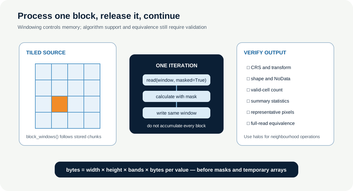
GeoTIFFs can be stored in tiles or scanline-like strips. src.block_shapes reports the preferred read chunks for each band. src.block_windows(1) yields block indices and corresponding windows for band 1.

Reading one cell from a tiled compressed file may require decoding its complete block. Repeated arbitrary tiny windows can therefore perform more I/O than following block boundaries.

Block shape is a storage property, not the scientific support of the measurement. A 64 × 64 tile does not become an ecological unit. Use blocks for efficient access while preserving the analytical method.

Check your understandingWhy process source block windows rather than arbitrary one-row reads?

Choose one answer

Block-aligned reads follow the file's efficient storage chunks and avoid repeated decodingA storage block is always the correct ecological supportBlocks eliminate the need for masks

Check answer

6. The read–calculate–write pattern limits memory

A windowed local transformation can follow:

1. open source and output once;
2. iterate source blocks;
3. read one masked block;
4. calculate the output for that block;
5. fill invalid cells with destination NoData;
6. write to the same window in the output;
7. release references and continue;
8. close and reopen the complete derivative;
9. compare it with the declared reference result.

Do not append every processed block to a list. That recreates full-array memory use. Aggregate only small diagnostics such as count, sum, minimum and maximum, using numerically appropriate methods.

7. Worked example — scale valid cells block by block

Predict before running

Should the output CRS, transform, shape and invalid-cell locations change when every valid value is multiplied by 100? What numerical relation must hold?

import rasterio

source_path = "data/raw/large_tiled_continuous.tif"
output_path = "outputs/large_tiled_scaled.tif"
with rasterio.open(source_path) as src:
    profile = src.profile.copy()
    with rasterio.open(output_path, "w", **profile) as dst:
        for _, window in src.block_windows(1):
            block = src.read(1, window=window, masked=True)
            scaled = block * 100
            dst.write(scaled.filled(src.nodata), 1, window=window)

Code walkthrough

1. Source and output paths remain different.
2. The source opens read-only.
3. The profile preserves the unchanged full-grid contract.
4. The destination remains open for the complete loop.
5. block_windows(1) follows stored band-1 blocks, including edge windows.
6. Each read carries the source mask.
7. Multiplication applies only to valid masked-array values.
8. Invalid cells are filled with the declared NoData for writing.
9. Each result is written into the corresponding full-grid window.
10. Leaving the context managers closes both datasets before verification.

The output stored values changed units or scale convention. Update tags and band descriptions so the factor is not hidden. If this were physical reflectance, confirm whether multiplication is a display scaling, a published scale factor or an invalid manipulation.

8. Neighbourhood operations need halos

The block-by-block pattern above is safe for a cell-independent multiplication. It is not sufficient for every algorithm.

Slope, convolution, focal mean and edge detection use neighbouring cells. A block computed without adjacent source cells creates seams at tile boundaries. Use a halo or overlap:

1. expand the read window by the required neighbourhood radius;
2. clip or use boundless handling at dataset edges;
3. calculate on the expanded block;
4. write only the central non-halo result to the destination window;
5. define edge behaviour and NoData propagation;
6. compare tile boundaries with a trusted full-array reference.

Global standardisation and histogram-based methods may require a first pass to calculate global statistics, followed by a second pass for transformation. Do not describe every algorithm as independently tileable.

Check your understandingWhy does a three-by-three filter need a halo around each write window?

Choose one answer

Cells at the window edge require neighbouring source values outside that windowA halo changes the source CRSEvery cell-independent multiplication requires one

Check answer

9. WarpedVRT provides a virtual transformed view

A GDAL virtual raster can present a dataset through another grid without immediately writing a full intermediate file. Rasterio's WarpedVRT configures that view with destination CRS, transform, width, height, NoData and resampling.

import rasterio
from rasterio.enums import Resampling
from rasterio.vrt import WarpedVRT

with rasterio.open("data/raw/different_crs.tif") as src:
    with WarpedVRT(src, crs=target_crs, transform=target_transform,
                   width=target_width, height=target_height,
                   nodata=target_nodata,
                   resampling=Resampling.bilinear) as vrt:
        preview = vrt.read(1, window=target_window, masked=True)
        print(vrt.crs, vrt.transform, preview.shape)

The virtual view performs transformation as data are requested. It can reduce unnecessary intermediates and support windowed access. It is not a persisted portfolio output. Record all VRT parameters, and write a final derivative when the workflow requires an immutable, independently inspectable product.

WarpedVRT does not remove the need to choose a scientifically defensible resampling method or target grid.

10. Equivalence checks depend on the operation

For exact cell-independent arithmetic, compare the windowed output with a full-array reference:

• identical CRS, transform, shape and NoData;
• identical valid mask;
• exact or tolerance-based value equality;
• equal valid count;
• equal sum, min, max and selected pixels;
• no seams at block boundaries;
• reopened output readable independently.

For floating calculations, use a declared absolute and relative tolerance informed by the method and data type. Do not use a loose tolerance simply to pass.

Checksum equality is useful when output bytes are expected to be deterministic and identical. Different compression or metadata ordering can change file checksums without changing values. A value-array checksum over a canonical encoding can be more relevant when exact numerical identity is required.

Check your understandingWhat must happen before comparing full and windowed runtime?

Choose one answer

Grid, mask and numerical results must pass declared equivalence checksThe faster method should be accepted automaticallyOnly output file sizes should be equal

Check answer

11. Measure time without turning the lesson into a race

Compare full and windowed methods under the same operation, environment and input. Record:

• Python, Rasterio, GDAL and NumPy versions;
• hardware and available memory;
• input checksum, dimensions, bands, type and block layout;
• whether file opening and writing are timed;
• warm-up and repeat count;
• elapsed time and estimated or measured peak memory;
• equivalence result;
• output size and compression.

For the tiny training raster, the full read may be faster because loop overhead dominates. That does not invalidate windowing for a large product. Report the scale and avoid universal speed-up claims.

12. Common mistakes and recovery

Equating compressed file size with RAM

Why it happens: storage size is visible. Recognition: no dimension × type calculation exists. Fix: estimate decompressed arrays and intermediates before reading.

Choosing arbitrary one-row windows

Why it happens: smaller windows seem memory efficient. Recognition: many repeated block decodes occur. Fix: inspect block shapes and choose windows aligned with storage and algorithm needs.

Accumulating all output blocks

Why it happens: results are kept for later concatenation. Recognition: a growing list recreates full memory use. Fix: write each completed block directly and retain only small audit summaries.

Ignoring edge and halo requirements

Why it happens: blocks are treated as independent arrays. Recognition: seams appear in terrain or filter outputs. Fix: expand reads, crop writes and compare boundaries with a full reference.

Treating WarpedVRT as a saved derivative

Why it happens: the virtual dataset behaves like an open raster. Recognition: downstream work depends on an undocumented transient configuration. Fix: record parameters and persist validated outputs when handover requires them.

Optimising before proving equality

Why it happens: time is easier to see than a subtle value difference. Recognition: benchmark tables omit mask and numerical comparisons. Fix: define correctness first and fail the benchmark when equivalence fails.

13. Guided practice — benchmark full and block-wise processing

Use large_tiled_continuous.tif.

1. record file checksum, profile and sixteen expected block windows;
2. estimate full array, mask and output memory;
3. implement valid-value multiplication by 100 with a full read;
4. implement the same operation using block_windows(1);
5. write both outputs under different names;
6. reopen both;
7. compare grids, masks, valid count, representative values and complete arrays;
8. calculate per-method elapsed time over several declared repetitions;
9. report estimated working memory and explain why the training timing cannot predict every system;
10. inspect block-edge rows and columns for seams;
11. create a small WarpedVRT window from different_crs.tif on the target grid;
12. export large_raster_processing_benchmark.csv.

Raster QA check

Load the full-read and block-wise derivatives in QGIS. Use a difference view or raster calculator to inspect whether valid cells differ. Check NoData edges, extent, pixel size and renderer. A zero-looking difference map is useful, but preserve the Python numerical assertion as proof.

14. Independent challenge — design for a raster larger than RAM

Write a processing plan for a four-band 40,000 × 40,000 float32 orthomosaic on a machine with 16 GiB RAM. The task applies a local three-by-three filter and writes a tiled GeoTIFF.

Your plan must include:

• value-array lower bound and realistic working-memory risks;
• selected block/window size and why;
• one-cell halo treatment;
• NoData and edge policy;
• output tiling and compression;
• progress and failure recovery;
• equivalence fixture small enough for a full read;
• metadata and representative-pixel checks;
• why Xarray and Dask are deliberately deferred rather than required here.

Scientific interpretation

Windowing and virtual views can make large-raster processing operationally feasible while preserving a declared result. They do not correct an invalid target grid, inappropriate interpolation or misunderstood variable. Efficiently producing the wrong raster remains a scientific failure.

15. Reflection, submission and portfolio artifact

Answer in your private notes:

1. Why can a small compressed GeoTIFF require large memory?
2. What information does block_windows() provide?
3. Which operations need halos or multiple passes?
4. When is a WarpedVRT useful, and when must an output be persisted?
5. What must be equal before performance results matter?

Submission

• Notebook: 06_large_raster_processing.ipynb with memory estimates, both implementations, WarpedVRT preview and equivalence tests.
• Table: large_raster_processing_benchmark.csv containing environment, block layout, timings, memory estimate and equality result.
• Screenshot: block layout or difference QA view with source and output metadata.
• Written answer: 220–300 words explaining the method, memory tradeoff and correctness evidence.

Portfolio artifact

Artifact 2.16 — Large-raster processing benchmark

Add the block-wise processor, equivalence test and conditional benchmark to the Raster QA and Harmonisation Pipeline. The pattern becomes the operational foundation for later UAV and satellite products.