Crop, Mask, Reproject and Resample

1. Name the operation before choosing the function

Learning outcome

By the end of this lesson, you will be able to distinguish crop, mask, reproject and resample operations; state which spatial property each changes; select a defensible resampling method from variable semantics; and produce a transformation decision log with reopened, validated raster outputs.

Prerequisites: Complete Lessons 2.11–2.12 and the earlier CRS and spatial-support lessons. You should be able to audit a raster, read a masked band and explain why a grid is more than shape. Allow 120–140 minutes. This is a concept and technical lab.

Why this matters

Raster processing conversations often use “clip,” “resize” and “project” loosely. Code then combines several changes in one call, and the output looks plausible. The analytical record no longer says whether values were removed, interpolated, moved to another reference system or merely cropped to a rectangle.

Use precise verbs:

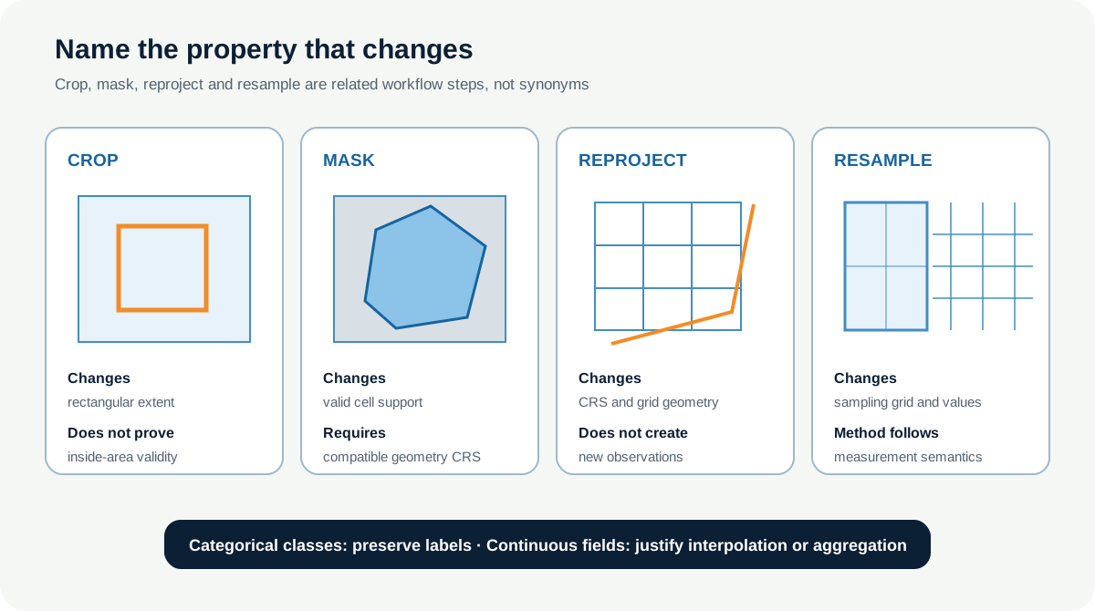
• crop changes rectangular extent;
• mask changes which cells are valid according to geometry or logic;
• reproject transforms coordinates and establishes a destination grid;
• resample estimates or assigns values on a different grid.

One workflow can require all four, but each must have its own reason and QA evidence.

Scientific rule: Resampling changes representation. It does not create observations or repair poor measurement quality.

Scientific context

The coastal-meadow team needs raster layers inside a synthetic site boundary and on one common analysis CRS. Continuous band-like values and categorical habitat codes respond differently to grid changes. A method that gives a smooth continuous surface can invent impossible habitat labels.

The files in the training pack expose these choices. They are synthetic. Their numerical patterns are designed to make errors visible, not to support ecological conclusions.

Learner action

Create 03_reprojection_resampling.ipynb. Before importing a processing function, make four rows labelled crop, mask, reproject and resample. For each, predict which of CRS, transform, extent, dimensions, valid support and values can change.

2. Crop changes the rectangular extent

A crop selects a rectangular window from a source grid. It can reduce rows, columns and bounds while preserving the source CRS and cell size. The output transform must move to the upper-left corner of the retained window.

A crop does not automatically exclude all cells outside an irregular study polygon. The bounding rectangle around a coastal boundary includes corners outside the site. Those cells remain present until a mask identifies them as invalid.

Windowed crop steps are:

1. express requested bounds in the raster CRS;
2. convert bounds to a window;
3. round or snap window offsets deliberately;
4. read that window;
5. calculate its transform with window_transform();
6. write new dimensions, bounds and transform;
7. reopen and compare the result with the requested rectangle.

“Clip to extent” in one tool may perform this rectangular crop. Record the actual behaviour rather than relying on the label.

Check your understandingWhat does a rectangular crop guarantee?

Choose one answer

A changed rectangular extent, not that every retained cell lies inside an irregular study areaAll cells outside a polygon are invalidThe raster has been reprojected

Check answer

3. Mask defines valid support

A polygon mask classifies cells according to their relationship with geometry. Depending on parameters, the result can keep the source extent and mark outside cells as NoData, or crop to the geometry's bounding box and then mask outside support.

Before masking:

• transform the geometry to the raster CRS;
• validate the geometry and its provenance;
• define whether boundary-touching cells count;
• decide between centre-based and all-touched behaviour;
• choose a destination NoData compatible with the data type;
• preserve the original source.

all_touched=False commonly selects cells whose centres lie within the geometry or that meet the rasterisation rule. all_touched=True includes every cell touched by the geometry, often increasing coverage along edges. Neither is universally correct. A narrow habitat boundary and a large cell can be highly sensitive to this choice.

Do not replace masked cells with zero unless zero has been declared as invalid for that variable and output contract. A masked cell means “not valid under this rule,” not “the measured quantity is zero.”

4. Reprojection transforms a grid, not only a CRS label

Reprojection connects two coordinate systems through a coordinate operation and creates values on a destination grid:

source grid → coordinate transformation → destination grid

The destination needs:

• CRS;
• transform and origin;
• resolution;
• width and height;
• bounds or extent policy;
• NoData policy;
• resampling method.

Changing the CRS metadata without recalculating coordinates is not reprojection. It is a false label. Raster reprojection also cannot preserve every source pixel value and footprint exactly because the destination grid usually intersects the source grid differently.

Rasterio's calculate_default_transform() can propose a destination transform and dimensions for a target CRS. That is a technical default, not necessarily the analysis grid you need. For stacking, a previously justified reference raster should often define the exact destination contract.

Check your understandingWhy is assigning a new CRS label not raster reprojection?

Choose one answer

Reprojection transforms coordinates and creates values on a destination gridA label always changes the stored pixel values correctlyRaster CRS metadata have no relationship to the transform

Check answer

5. Resampling follows measurement semantics

Resampling assigns or estimates values when source and destination cells do not coincide. There is no universally best method.

Nearest neighbour

Nearest neighbour assigns the value of a nearby source cell. It preserves existing categorical labels and is the default choice for land-cover or habitat class codes. It can produce blocky continuous surfaces and does not perform aggregation when coarsening.

Bilinear interpolation

Bilinear uses a weighted combination of nearby source values. It can be suitable for continuous surfaces when local interpolation matches the variable and intended use. It smooths values and is not class-preserving.

Cubic interpolation

Cubic uses a wider neighbourhood and a smoother function. It may overshoot the source range and create values below or above valid limits. Use it only with evidence and post-resampling range checks.

Average for aggregation

When coarsening a continuous raster, average can summarise contributing source cells. Its result depends on valid coverage, weighting and support. An average of reflectance-like values is not automatically the same physical observation a coarser sensor would have made.

For categorical downsampling, a mode-like method may be appropriate for dominant class, but it changes the estimand and can erase rare classes. Record tie handling and valid coverage.

Variable	Typical starting method	Required caution
habitat class codes	nearest	preserves labels, not class area proportions
continuous elevation surface	bilinear or cubic under stated use	smoothing, overshoot and edge effects
continuous values coarsened to larger cells	average under stated support	mask and partial-coverage handling
quality flags or bit masks	nearest	integer codes may encode several bits

Check your understandingWhich starting rule is defensible for habitat class codes?

Choose one answer

Use nearest neighbour and verify valid output labels against the legendUse bilinear because smoother boundaries are more accurateUse cubic because it always preserves source range

Check answer

6. Predict before running — class codes expose the mistake

Imagine adjacent habitat cells with labels 1 and 3. A bilinear calculation can produce 1.5, 2.0 or 2.5. Unless the legend defines those values, the outputs have no categorical meaning. Rounding them afterward invents a rule that was not part of the classification.

Predict the consequences:

1. 10 m habitat raster → 5 m with bilinear;
2. 10 m continuous surface → 20 m with average;
3. polygon mask applied while geometry remains in another CRS;
4. 10 m raster → 1 m with any interpolation.

The first creates invalid class mixtures. The second can provide a larger-support summary if masks and coverage are handled. The third can create no overlap or mask the wrong region. The fourth creates more output cells, not more observed detail.

7. Worked example — make resampling explicit

Before running, predict which layer should use nearest and which may use bilinear. Do not interpret the printed names as proof that the methods are appropriate for every future product.

from rasterio.enums import Resampling

resampling_plan = {
    "habitat_class": Resampling.nearest,
    "red_reflectance_proxy": Resampling.bilinear,
    "nir_reflectance_proxy": Resampling.bilinear,
    "dsm_surface": Resampling.bilinear,
}

for variable, method in resampling_plan.items():
    print(f"{variable}: {method.name}")

Code walkthrough

1. Resampling provides Rasterio/GDAL method identifiers instead of ambiguous strings.
2. The plan is keyed by variable meaning, not filename alone.
3. The categorical habitat codes use nearest neighbour to preserve labels.
4. The synthetic continuous band proxies use bilinear as a declared instructional choice.
5. The DSM is treated as a continuous surface, but its scientific interpretation remains constrained by surface meaning and vertical metadata.
6. The loop prints the decision record before processing.

The dictionary is incomplete until you add source resolution, target resolution, extent, mask rule, justification, expected numerical consequence and QA test.

8. Reproject one raster into an explicit target array

Rasterio's reproject() separates source and destination grids. The destination array must be created with a deliberate data type and fill value.

import numpy as np
from rasterio.warp import reproject

destination = np.full(target_shape, target_nodata, dtype="float32")
reproject(
    source=source_band,
    destination=destination,
    src_transform=source_transform,
    src_crs=source_crs,
    src_nodata=source_nodata,
    dst_transform=target_transform,
    dst_crs=target_crs,
    dst_nodata=target_nodata,
    resampling=Resampling.bilinear,
)

This cell assumes the source and target variables shown above have already been defined from audited datasets. The explicit source NoData prevents invalid sentinel values from being interpolated as measurements. The target transform, CRS and shape—not only dst_crs—define the output grid.

For a categorical raster, change the destination type and use Resampling.nearest. Afterward, verify that unique valid outputs remain within the source class legend.

9. Mask with a geometry in the raster CRS

Rasterio's mask function can apply a GeoJSON-like geometry:

import rasterio
from rasterio.mask import mask

with rasterio.open("data/raw/source.tif") as src:
    masked, masked_transform = mask(
        src, [study_geometry], crop=True,
        all_touched=False, nodata=src.nodata,
        filled=False,
    )

print(masked.shape, masked_transform)

study_geometry must already be in src.crs. crop=True reduces the rectangular extent to the geometry bounds, while the mask still marks cells outside the polygon. filled=False keeps a masked array rather than immediately substituting the NoData value.

Compare all_touched=False and True only as a sensitivity test with a stated support rationale. Do not choose the option that gives the preferred mean.

Check your understandingWhat must be true before a polygon mask is applied to a raster?

Choose one answer

The geometry must be valid and transformed into a compatible raster CRSThe polygon and raster need only share a filename prefixEvery outside cell must be replaced by numeric zero

Check answer

10. Build a transformation decision log

Record one row for each operation, even if several happen in one function call:

Field	Example question
input and checksum	Which immutable source was used?
operation	Crop, mask, reproject or resample?
scientific purpose	Why must this property change?
source contract	CRS, transform, shape, bounds, NoData, semantics?
target contract	Which explicit destination grid is required?
method and parameters	Bounds, geometry, resampling, all-touched rule?
expected change	Which metadata and values may differ?
invariant	Which identity, class labels or support must be preserved?
output path	Which named derivative was created?
validation	Which reopened checks passed?
limitation	Which information cannot be recovered?

Operation order matters. Reprojecting a full large raster and then cropping may cost more than transforming the requested bounds and reading an appropriate subset. Masking before or after reprojection can produce edge differences because the grids differ. State the chosen sequence and validate boundary sensitivity.

11. Common mistakes and recovery

Calling every extent operation a clip

Why it happens: GIS interfaces use overlapping labels. Recognition: the report does not say whether outside-polygon cells remain. Fix: record rectangular crop and geometry mask as separate effects.

Changing a CRS label instead of reprojecting

Why it happens: the layer appears in a new coordinate system immediately. Recognition: transform numbers are unchanged despite a new CRS. Fix: recover the verified source CRS and run a coordinate transformation to an explicit destination grid.

Interpolating categories

Why it happens: bilinear output looks smooth. Recognition: new non-integer or undefined class values appear. Fix: use a class-preserving method and verify unique outputs against the legend.

Treating upsampling as enhanced resolution

Why it happens: output cells are smaller. Recognition: claims of added detail appear without new observations. Fix: describe it as resampling to a finer grid and retain native-resolution limitations.

Letting invalid cells influence interpolation

Why it happens: NoData is not passed to the warp. Recognition: extreme halos appear near missing regions. Fix: declare source and destination NoData, then compare mask boundaries.

Trusting the default output grid

Why it happens: software proposes dimensions automatically. Recognition: origin and extent vary between runs or layers. Fix: define a justified target contract and reuse it for every stack member.

12. Guided practice — perform four traceable operations

Use aligned_continuous.tif, training_site_boundary.geojson and one raster that differs from the target.

1. inventory and checksum every source;
2. transform the site geometry to the raster CRS;
3. crop the continuous raster to a declared rectangle and record the new transform;
4. mask it to the study polygon, comparing the two all-touched rules;
5. reproject different_crs.tif into the exact aligned_continuous.tif grid;
6. resample different_resolution.tif into that same grid with a continuous method;
7. resample the aligned categorical raster to a finer test grid with nearest neighbour;
8. deliberately try bilinear into a floating test array and list the invalid class values;
9. write every accepted derivative to a new file;
10. reopen and compare CRS, transform, shape, bounds, NoData, class labels and representative valid values;
11. export raster_transformation_decision_log.csv;
12. delete only temporary experimental arrays, not source evidence or accepted derivatives.

Raster QA check

In QGIS, load source and derivative layers. Compare the crop rectangle with the polygon mask, toggle transparency at mask edges and inspect class values with Identify. Confirm that visual alignment agrees with the numerical grid record. Record edge differences and renderer settings; do not use appearance as the alignment assertion.

13. Independent challenge — review a requested “resolution improvement”

A collaborator asks you to turn a 20 m habitat raster into a 1 m raster “so it matches the UAV accuracy.” Write a technical response before processing:

• distinguish pixel size, resolution and accuracy;
• explain why bilinear is invalid for class codes;
• explain what nearest-neighbour upsampling would and would not change;
• propose a target-grid decision based on the analysis question;
• state how class boundaries and rare classes may be affected;
• define validation evidence and a limitation statement.

Create a small synthetic demonstration with nearest and bilinear outputs. Do not present either as improved thematic accuracy.

Scientific interpretation

These operations can create a consistent representation for analysis under a declared grid and support rule. They cannot recover information absent from the source, validate incorrect CRS metadata, improve original positional accuracy or make different sensors observe the same phenomenon. Harmonisation is a controlled compromise, not a truth-generating step.

14. Reflection, submission and portfolio artifact

Answer in your private notes:

1. How does a crop differ from a mask?
2. Why does reprojection usually require resampling?
3. Which evidence determines whether bilinear is defensible?
4. What does upsampling change, and what remains unchanged?
5. Why must source NoData be passed into a warp?

Submission

• Notebook: 03_reprojection_resampling.ipynb containing four traceable operations and the categorical demonstration.
• Table: raster_transformation_decision_log.csv with inputs, target grid, method, expected change and reopened validation.
• Screenshot: source, crop, mask and aligned derivative compared in QGIS.
• Written answer: 240–320 words justifying the operation sequence and resampling choices while stating what the output does not improve.

Portfolio artifact

Artifact 2.13 — Raster transformation decision log

Add the accepted derivatives and decision log to the Raster QA and Harmonisation Pipeline. This record becomes the provenance link between raw rasters and the common-grid validation in Lesson 2.14.