Point Clouds, DSM, DTM and Orthomosaics

1. Product names do not prove product meaning

Learning outcome

By the end of this lesson, you will be able to distinguish sparse and dense point clouds, photogrammetric and LiDAR attributes, DSM and DTM, orthorectified imagery and orthomosaics; explain seamlines, occlusion, resampling and edge effects; and evaluate whether surface differencing supports a canopy-height interpretation.

• Lesson type: Scientific product lab
• Estimated time: 110–130 minutes
• Prerequisites: Lesson 2.17 terrain concepts and Lesson 2.22 reconstruction workflow.

Why this matters

UAV handovers often contain an orthomosaic and DSM with little explanation. Their names can encourage unsupported conclusions: “DSM equals canopy,” “DTM equals true terrain,” or “orthomosaic pixels are raw measurements.” A scientist must identify how each product was derived, what surface or image contribution it represents and where uncertainty enters.

Scientific context

The synthetic pack contains an RGB mosaic preview, a smooth DSM and a DSM with a spike and pit. It deliberately provides no validated DTM. Therefore, the correct lesson outcome is not to calculate canopy height. It is to explain what additional ground-surface and vertical evidence would make such a calculation defensible.

Mental model

Learner action

Create 06_uav_products.ipynb. Begin a table with columns product, direct or derived, input evidence, spatial meaning, main uncertainty, appropriate use and prohibited interpretation.

2. Sparse and dense point clouds serve different stages

A sparse point cloud contains reconstructed tie points from feature correspondences. It supports camera alignment, block diagnosis and initial three-dimensional geometry. Its density follows detectable features and filtering.

A dense point cloud estimates many more surface points after the camera model is established. It supports surface, mesh and orthomosaic generation. Density depends on image GSD, texture, algorithm, quality settings, view geometry and filtering.

Neither cloud is a direct continuous surface. Both contain discrete points with uneven density and uncertainty. A dense cloud can be detailed but wrong in water, moving vegetation or poorly matched edges.

Useful point-cloud attributes may include:

• X, Y and Z coordinates;
• RGB sampled from imagery;
• classification or class confidence;
• image observations or confidence scores;
• normals or processing quality fields.

LiDAR may add return number, number of returns, intensity, scan angle and classification. Photogrammetric RGB and LiDAR intensity are not equivalent measurements. A photogrammetric cloud does not inherit LiDAR return penetration through canopy.

Check your understandingWhat primarily distinguishes a sparse SfM cloud from a dense reconstruction?

Choose one answer

Sparse points come from tie-point geometry; dense processing estimates many more surface pointsSparse clouds are always LiDARDense clouds are continuous terrain truth

Check answer

3. A DSM represents the reconstructed upper visible surface

A digital surface model (DSM) grids the upper surface represented by source points or mesh. In UAV photogrammetry it may include:

• vegetation canopy;
• buildings, fences and equipment;
• exposed ground;
• water-edge failure;
• interpolated holes;
• spikes, pits and noisy moving vegetation;
• smoothing introduced by dense-cloud or gridding settings.

The cell value is not automatically the highest true object. It reflects the reconstruction and gridding rule. Units and vertical reference must be documented separately from horizontal CRS.

The clean synthetic DSM represents a plausible upper surface with an undocumented vertical datum. It is suitable for practising metadata and local-consistency checks, not for real elevation claims.

4. A DTM is an interpreted terrain approximation

A digital terrain model (DTM) represents estimated bare-earth terrain. Creating one requires identifying ground points and interpolating across non-ground areas. The method may use classification, filtering, breaklines, external terrain data or manual review.

In dense vegetation, photogrammetry often sees canopy rather than ground. A DTM derived only from those images can be poorly supported. Interpolation can appear smooth while spanning areas with no ground observations.

Ask:

• which points were classified as ground and how;
• ground-point density and distribution;
• interpolation method and search distance;
• validation against independent elevations;
• treatment of channels, banks and breaklines;
• vertical datum, units and epoch;
• whether “DTM” is only a filename label.

Check your understandingWhat evidence is required before calling a product a DTM?

Choose one answer

A documented ground-identification, interpolation and validation processA smooth elevation surfaceThe filename contains terrain

Check answer

5. A canopy-height model is a conditional difference

The common relationship is:

CHM = DSM − DTM

This difference can support canopy-height interpretation only when:

• DSM and DTM grids align cell by cell;
• horizontal and vertical references match;
• units and scale agree;
• surfaces represent appropriate dates;
• the DSM captures the relevant canopy surface;
• the DTM estimates ground under that canopy;
• artefacts and uncertainty are assessed.

Even then, a raster difference may represent surface separation rather than individual plant height. Salt-meadow vegetation can be below pixel and reconstruction sensitivity. Wind and surface smoothing can bias height.

The synthetic pack contains no DTM. Subtracting an arbitrary constant or relabelling the DSM is prohibited. Record DTM evidence missing as a stop condition.

6. Orthorectification removes modelled perspective displacement

Orthorectification maps source-image pixels to ground coordinates using:

• estimated camera position and orientation;
• internal camera model;
• a chosen surface model;
• output CRS and grid;
• resampling rule.

A surface-height error creates planimetric displacement, especially away from the image centre and for tall objects or oblique views. Using a bare-earth terrain model to rectify imagery over trees can shift canopy tops; using a noisy DSM can distort texture.

Orthorectification is not the same as assigning or transforming a CRS. It models perspective geometry and relief. Reprojection changes coordinate representation of an already georeferenced product.

Worked example — detect local DSM anomalies

Predict before running

Will a global mean clearly expose one spike and one pit in a 40 × 40 surface?

import rasterio
import numpy as np

with rasterio.open("data/raw/uav_dsm_spike_demo.tif") as src:
    dsm = src.read(1, masked=True)

median = np.ma.median(dsm)
deviation = np.ma.abs(dsm - median)
suspect = (~np.ma.getmaskarray(dsm)) & (deviation.data > 5)

print("range:", float(dsm.min()), float(dsm.max()))
print("suspect cells:", int(suspect.sum()))
print("indices:", np.argwhere(suspect))

Code walkthrough

1. Rasterio reads values with the declared NoData mask.
2. The median provides a robust whole-fixture reference, not a universal terrain model.
3. Absolute deviation measures difference from that reference.
4. The mask excludes invalid support.
5. Five metres is a predeclared synthetic-fixture threshold.
6. Range reveals the -3 m pit and 18.5 m spike.
7. Indices locate cells for spatial diagnosis.
8. Real DSM QA needs local terrain/structure context; a global threshold can flag true tall objects.

7. An orthomosaic combines multiple orthorectified images

An orthomosaic is built from image pieces projected to a common grid. The software chooses contributions, seamlines, colour balancing and blending. Different cells can come from different source images and times.

Useful provenance includes:

• source image contribution or seamline layer;
• acquisition time per source region;
• orthorectification surface;
• output grid and resampling;
• radiometric correction and colour balancing;
• excluded frames and masks;
• mosaic blending parameters.

The synthetic RGB preview has a brightness seam near column 21 and locally shifted texture near it. It is an 8-bit display product, not reflectance. The seam can be radiometric, while ghosting can indicate geometric or temporal disagreement.

Check your understandingWhy can one orthomosaic contain a visible seam?

Choose one answer

Different orthorectified source images can differ in illumination, geometry, time or sharpnessEvery source pixel is one simultaneous exposureThe DSM is necessarily bare earth

Check answer

8. Seamlines and ghosting have causes

A seamline is a boundary between source-image contributions. It can be visible because:

• exposure or illumination differs;
• vegetation moved;
• view-dependent response differs;
• orthorectification surfaces displace features differently;
• source sharpness differs;
• colour balancing is incomplete.

Ghosting occurs when one object or edge appears duplicated or smeared because contributions do not align. It may reflect moving objects, vegetation motion, geometry error, surface mismatch or blending.

Not every visible seam invalidates analysis. If a seam changes display tone only in an RGB visual product, it may be cosmetic for one use. If it changes calibrated band values or crosses target plots, it can bias extraction. Connect defect to variable and support.

9. Occlusion, edge geometry and interpolation

An object hidden from a camera viewpoint is occluded. Multiple views can reduce occlusion, but dense canopy, banks and structures still hide surfaces. A DTM cannot recover unseen ground without a model or other data.

Block edges have fewer observations and narrower view geometry. Dense clouds can become noisy or sparse; orthomosaic features can shift. Include acquisition margins and inspect product quality beyond the analysis boundary.

Interpolation fills gaps according to an algorithm. It creates estimates, not observations. Report filled regions and maximum gap distance. A smooth DSM across water or dense canopy can be numerically convenient but scientifically unsupported.

10. Resampling changes the final raster representation

During orthorectification and mosaicking, source pixels contribute to output cells through nearest, bilinear, cubic or other rules. A chosen output GSD can differ from source-image nominal GSD.

Creating 1 cm output cells from 2.2 cm source GSD does not create new detail. Multiple views can improve reconstruction or reduce noise under some conditions, but output pixel count is not independent information.

For continuous radiometric products, interpolation may be justified; for categorical masks, nearest neighbour often preserves labels. Always record method and validate range, mask and edge behaviour.

QA check

Compare source nominal GSD, orthomosaic pixel size and effective feature sharpness. If the output grid is finer, describe it as oversampled unless evidence supports increased resolved detail.

11. Common mistakes and recovery

DSM equals DTM

Why: both are elevation grids. Detect: ground classification is absent. Recover: verify surface meaning and ground evidence.

DSM equals vegetation height

Why: canopy appears high. Detect: no aligned DTM or vertical validation. Recover: treat DSM as upper surface and require a defensible terrain estimate.

Orthomosaic equals raw photograph

Why: it looks photographic. Detect: seams and orthorectification history are ignored. Recover: document contributions, surface, resampling and time.

Smooth surface means accurate surface

Why: artefacts are less visible. Detect: interpolation and filters are undocumented. Recover: inspect point support, gaps and independent elevations.

Fine output pixels mean fine information

Why: the file reports small resolution. Detect: output size is compared without source geometry. Recover: report nominal source GSD, processing and effective resolution.

12. Guided practice — product interpretation table

1. Inventory uav_rgb_preview.tif, uav_dsm.tif and uav_dsm_spike_demo.tif.
2. Record bands, type, NoData, CRS, transform, resolution, bounds and units.
3. Label RGB as display values and DSM as a reconstructed upper surface.
4. Compare clean and defective DSM cell by cell.
5. Locate spike and pit and inspect surrounding pattern.
6. Compare left/right RGB brightness around the seam.
7. Inspect the ghosted patch at large scale.
8. State which source or processing evidence is absent for orthorectification.
9. Write why no canopy-height model can be created.
10. Complete the product table with appropriate and inappropriate interpretations.
11. Assign accept/review/unsuitable separately for visual context, surface analysis and plot extraction.
12. Reopen exported tables and preserve checksums.

QGIS visual QA companion

Display the clean and defective DSM with the same elevation stretch and hillshade settings. Blink the RGB mosaic around the seam and overlay the field polygons. Record whether defects intersect analytical support. Do not edit the raw fixtures.

QA checklist

• Sparse and dense point clouds are distinguished.
• Photogrammetric and LiDAR attributes are not conflated.
• DSM and DTM meanings are evidence-based.
• Vertical units/reference and grid alignment are explicit.
• Orthorectification surface and resampling are recorded.
• Seamline, ghosting, occlusion and edge support are inspected.
• Filled or smoothed areas are traceable.

13. Independent challenge — assess a proposed canopy product

A contractor provides a 3 cm orthomosaic and 5 cm DSM. They subtract a 1 m public terrain model acquired eight years earlier and call the result “plant height.” Write a technical assessment covering grid alignment, horizontal and vertical reference, dates, surface meanings, vegetation visibility, interpolation, support, expected accuracy and validation. Decide what can be retained and what must be renamed or rejected.

Scientific interpretation

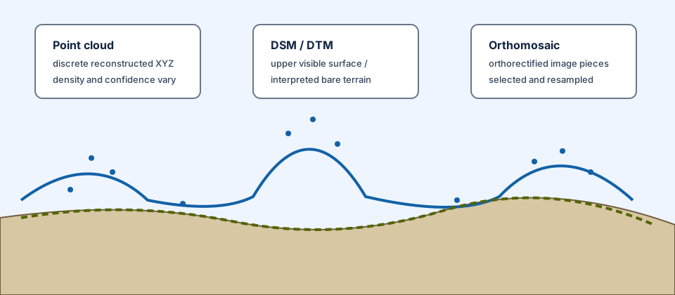
UAV products represent different stages of a modelled evidence chain. A point cloud is discrete; a DSM is an estimated upper surface; a DTM is an interpreted ground surface; an orthomosaic is a multi-image, surface-corrected raster. Product names are hypotheses about meaning that provenance and QA must support.

14. Reflection, submission and portfolio artifact

Answer in your private notes:

1. How do sparse and dense clouds differ?
2. What does a DSM represent?
3. What evidence makes a DTM credible under dense vegetation?
4. Why can orthomosaics contain seamlines?
5. When can DSM − DTM support canopy-height interpretation?

Submission

• Notebook: 06_uav_products.ipynb with DSM and mosaic diagnostics.
• Table: product interpretation matrix.
• Map: seam/ghost and DSM anomaly locations.
• Written answer: 280–350 words explaining why the supplied DSM is not a DTM or direct height.

Portfolio artifact

Artifact 2.23 — UAV product interpretation table

Add the table and spatial diagnostics to the Professional UAV Product Audit and Processing Report.