GeoPandas and Spatial Tables

1. Treat every spatial layer as a table with a contract

Learning outcome

By the end of this lesson, you will be able to read a vector file as a GeoDataFrame, explain how geometry and CRS extend an ordinary pandas table, filter features without losing spatial meaning, inspect feature and dataset bounds, create a diagnostic plot, and write a verified GeoPackage derivative. You will add a reusable vector-layer audit to the UAV and Satellite Analysis Pipeline.

Prerequisites: Complete Lessons 2.1–2.4. You should understand vector geometry, CRS evidence, scale and format choice, and be comfortable filtering a pandas DataFrame. Allow 90–120 minutes.

Why this matters

Vector files often open without complaint even when they contain duplicate identifiers, unexpected geometry types, empty features or implausible coordinates. A quick map may look reasonable because plotting software chooses an extent around whatever coordinates it receives. That visual success does not establish that the layer represents the intended locations or can support the next operation.

A professional analyst therefore performs a spatial audit before analysis. The audit answers three connected questions:

1. What does one feature represent?
2. Which geometry and reference system locate it?
3. Which evidence shows that the features are complete, unique and plausible?

This habit prevents errors from propagating into buffers, joins, raster extraction and modelling.

Core spatial question: What does each row represent, and how does its geometry relate to its attributes?

Scientific context

The published Baltic plant-traits table does not include plot coordinates. It must not be turned into a map by inventing locations. For Lessons 2.5–2.7, the research group provides a separate synthetic vector training pack. Its points and boundaries are deliberately constructed to reveal boundary, unmatched-feature and one-to-many cases.

These training features are not published sampling sites and cannot support ecological conclusions. Their role is to let you learn a professional method before applying it to governed field coordinates.

Download the four GeoJSON files and their README. Place them under:

data/training/vector_foundations/

Keep the filenames unchanged. Read the README before opening a file.

Learner action

Add ## Lesson 2.5 — GeoPandas and spatial tables to the continuing Module 2 notebook. Record the data status in one sentence: synthetic instruction, not published field evidence. Then write what you expect one row of training_field_plots.geojson to represent.

2. A GeoDataFrame extends pandas

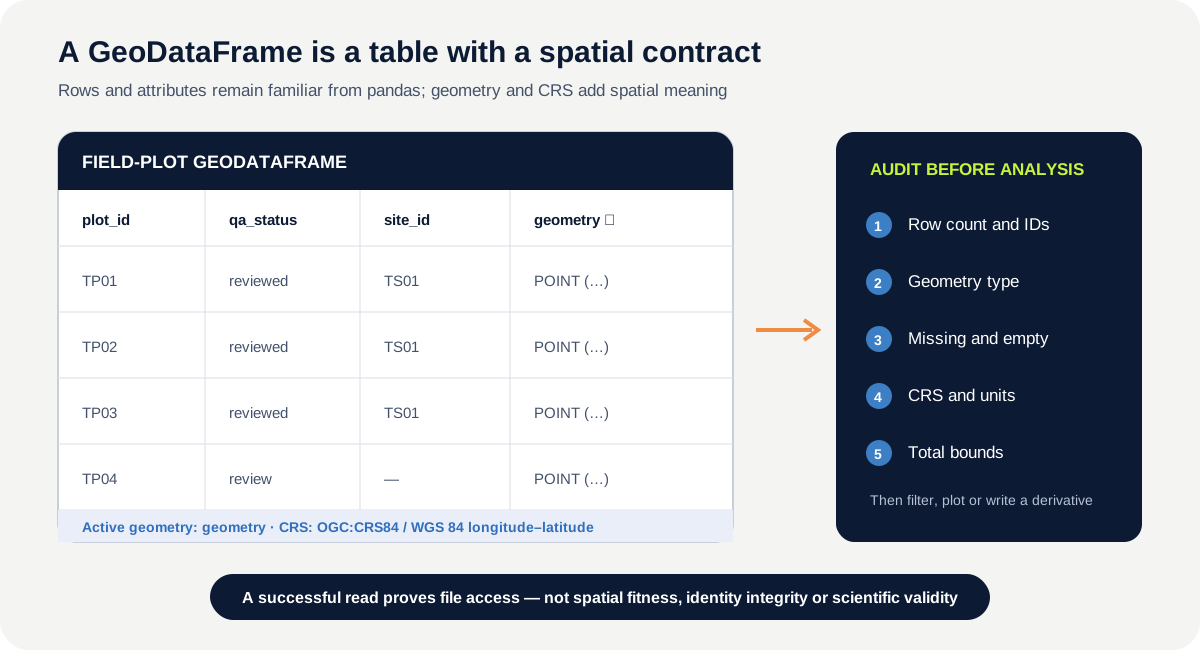
A pandas DataFrame organises rows and named columns. A GeoDataFrame keeps that tabular structure and adds spatial behaviour. It contains at least one column that stores Shapely geometry, and one geometry column is designated as active.

The active geometry determines what operations such as plotting, bounds, reprojection and spatial joins use. A GeoDataFrame can contain another geometry-valued column, but only the active one drives those operations until you deliberately switch it.

Four components should remain conceptually separate:

Component	Meaning	Audit question
index	pandas row label	Is it stable, unique and meaningful, or only a temporary row index?
identifier column	domain or workflow identity	Does plot_id uniquely identify the intended feature?
attributes	measured or descriptive values	Are types, missingness and categories plausible?
active geometry + CRS	spatial representation	What geometry is stored, and how do its coordinates relate to Earth?

Do not use the DataFrame index as a scientific identifier unless the data contract explicitly makes it one. File readers may create or reorder indexes. A stable column such as plot_id is easier to validate and preserve across formats.

Check your understandingWhat makes a GeoDataFrame spatial rather than an ordinary pandas DataFrame?

Choose one answer

An active geometry column and CRS connect tabular records to a spatial representationEvery column must contain coordinatesIts index automatically becomes a scientifically stable feature identifier

Check answer

3. Read a vector file without treating access as validation

GeoPandas uses gpd.read_file() to read formats supported by its I/O engine and GDAL/OGR. A successful call establishes that the software could interpret the file structure. It does not prove that the CRS label is true, that all components were delivered, or that the feature identity is correct.

The training pack uses GeoJSON. Under RFC 7946, GeoJSON positions use WGS 84 longitude and latitude in decimal degrees, with longitude first. GeoPandas normally reports a compatible geographic CRS. Inspect the result; do not assign a different CRS merely because a later operation requires metres.

Use a project-relative path built with pathlib.Path. This keeps the notebook portable:

project/
├── data/
│   └── training/vector_foundations/
├── outputs/
└── UAV_Satellite_Analysis_Pipeline.ipynb

Before reading, verify the path you are about to use. After reading, record the exact filename and package environment. A notebook that silently reads another copy with the same filename is not reproducible.

4. Audit feature identity and geometry

Begin with checks that can stop the workflow:

• row count: compare with the handover manifest;
• stable ID: report missing and duplicated plot_id values;
• geometry type: confirm that a plot layer contains points rather than a mixture of points and polygons;
• missing geometry: geometry.isna() identifies records without a geometry object;
• empty geometry: geometry.is_empty identifies geometry objects that contain no coordinates;
• CRS: inspect the stored definition and units;
• bounds: check coordinate ranges against the documented study region and reference system.

Missing and empty geometry are not the same. Missing means no geometry value is present. Empty means a geometry object exists but represents an empty set. Both require a documented decision, but their causes can differ.

Geometry validity is developed in Lesson 2.6. For a first audit, record validity rather than automatically repairing anything. A repair can change geometry type, parts or area and must be treated as a transformation.

5. bounds and total_bounds answer different questions

gdf.bounds returns four values for every feature: minimum x, minimum y, maximum x and maximum y. It is useful for detecting a single outlying geometry.

gdf.total_bounds returns one four-value envelope for the whole layer. It is useful for a rapid dataset-level extent check.

Neither proves positional accuracy. A layer can have plausible total bounds while individual points are swapped, shifted or assigned to the wrong site. Use both scales of evidence:

1. compare total_bounds with the declared delivery extent;
2. inspect per-feature bounds or representative coordinates;
3. compare against an independent authoritative reference when locations matter.

For geographic longitude–latitude data, the values are angular degrees. Do not interpret envelope width or height as metres.

6. Filter without breaking the spatial contract

Boolean filtering works as it does in pandas:

reviewed = plots.loc[plots["qa_status"] == "reviewed"].copy()

The result remains a GeoDataFrame because the active geometry is retained. .copy() makes the intention to create an independent working subset explicit and avoids confusing later modifications.

Filtering is a scientific decision when it changes the analysis population. Record:

• the rule;
• the number and IDs retained;
• the number and IDs excluded;
• why exclusion is justified;
• whether the raw layer remains unchanged.

Do not delete a boundary or outlying case merely because it complicates the map. In this training pack, those cases are deliberately preserved because they test the workflow.

7. Plot for diagnosis, not proof

gdf.plot() provides a fast diagnostic view. It can reveal a gross outlier, an unexpected geometry type or an empty layer. Add a boundary layer and use different styling for reviewed and unresolved records.

A diagnostic plot should have:

• equal axis scaling where appropriate;
• a title stating that the data are synthetic;
• distinct styles for QA categories;
• axes or contextual reference sufficient to identify the coordinate space;
• no decorative basemap presented as validation.

Plotting libraries can make unverified data look precise. The map supports inspection; the numerical audit remains the reproducible evidence.

Check your understandingWhich evidence should be recorded before using a newly opened point layer?

Choose one answer

Row and ID checks, geometry types, missing and empty geometry, CRS and boundsOnly a screenshot showing that the points drawOnly the file extension and modification date

Check answer

8. Worked example — produce a compact spatial audit

Before running, predict the row count, geometry type, CRS and whether any plot_id is duplicated. Which result would make you stop before plotting?

from pathlib import Path
import geopandas as gpd

path = Path("data/training/vector_foundations/training_field_plots.geojson")
plots = gpd.read_file(path)
audit = {
    "rows": len(plots),
    "crs": str(plots.crs),
    "geometry_types": plots.geom_type.value_counts().to_dict(),
    "missing_geometry": int(plots.geometry.isna().sum()),
    "empty_geometry": int(plots.geometry.is_empty.sum()),
    "duplicate_ids": int(plots["plot_id"].duplicated().sum()),
    "total_bounds": plots.total_bounds.round(5).tolist(),
}
print(audit)

The expected audit has five point features, no missing or empty geometry, no duplicated plot_id, a WGS 84-compatible geographic CRS and longitude–latitude bounds covering the synthetic training extent.

Code walkthrough

1. Path creates an operating-system-safe project-relative path.
2. geopandas is imported with its standard gpd alias.
3. path records the precise training input rather than searching the computer for a filename.
4. read_file() returns a GeoDataFrame and selects its geometry column.
5. audit stores named evidence so results can later be exported or compared.
6. len(plots) counts input features.
7. str(plots.crs) records the parsed spatial reference without assuming its display wording.
8. geom_type.value_counts() reveals unexpected geometry mixtures.
9. isna() counts missing geometry values.
10. is_empty counts geometry objects with no spatial content.
11. duplicated() checks the stable workflow identifier, not the temporary DataFrame index.
12. total_bounds records the layer envelope; rounding improves reporting, not the underlying coordinates.
13. print() exposes the complete audit for comparison with your prediction.

If any stop condition fails, keep the input unchanged and investigate. Do not continue simply because the next code cell can run.

9. Write a derivative and verify the round trip

After the raw GeoJSON passes the required checks, transform a copy to the justified analysis CRS and write a GeoPackage derivative:

analysis = plots.to_crs("EPSG:3301")
output = Path("outputs/vector_foundations.gpkg")
analysis.to_file(output, layer="training_field_plots", driver="GPKG")
reopened = gpd.read_file(output, layer="training_field_plots")
print(len(reopened), reopened.crs, reopened.total_bounds)

The write is not complete until the derivative is reopened and compared. Verify row count, stable IDs, geometry types, CRS and bounds. Because reprojection changes coordinate values, compare Earth location through an independent reference or transformation round trip—not by expecting identical numbers.

Use a new output path. The GeoJSON training input is raw instructional evidence and should remain immutable.

Check your understandingWhen is the new GeoPackage derivative ready for analytical use?

Choose one answer

After it is reopened and row count, IDs, geometry, CRS and bounds are compared with the intended source transformationWhen to_file() returns without raising an exceptionWhen its file size is smaller than the GeoJSON input

Check answer

10. Common mistakes and recovery

Treating the map as the audit

Why it happens: spatial patterns are easier to notice visually. Recognition: the notebook contains a plot but no row, ID, geometry or CRS report. Fix: run and preserve a numerical audit before interpreting the map.

Assuming the index is the plot identifier

Why it happens: the index appears beside every row. Recognition: identity changes after filtering or file conversion. Fix: validate a stable identifier column and reset the index only as a table operation, not as scientific identity.

Confusing missing with empty geometry

Why it happens: both may disappear from a map. Recognition: only one condition is checked. Fix: report isna() and is_empty separately and investigate their different provenance.

Measuring geographic bounds in metres

Why it happens: the four bound values look like ordinary coordinates. Recognition: longitude–latitude differences are labelled as metres. Fix: inspect CRS units and transform a copy to a justified projected CRS before distance or area analysis.

Overwriting the source during export

Why it happens: a new format feels like a better version. Recognition: the original handover can no longer be reproduced. Fix: keep raw data immutable and write a named derivative under outputs/ with a processing record.

11. Guided practice — audit the complete training handover

Apply one reusable audit function or repeated audit block to:

1. training_field_plots.geojson;
2. training_study_area.geojson;
3. training_management_zones.geojson;
4. training_vegetation_zones.geojson.

For each layer:

1. record path and SHA-256 checksum or another documented integrity identifier;
2. report row count and stable identifier field;
3. check missing and duplicated identifiers;
4. report geometry types, missing geometry, empty geometry and validity count;
5. record CRS and total_bounds;
6. inspect per-feature bounds for outliers;
7. create one diagnostic plot with the synthetic status visible;
8. transform a copy to EPSG:3301 and record the target bounds and units;
9. write all four derivatives as named layers in one GeoPackage;
10. reopen every layer and compare the audit with the in-memory source.

Required QA evidence

Submit one table with a row for each layer and columns for source, checksum, feature count, ID field, duplicates, geometry types, missing, empty, invalid, CRS and total bounds. Include a separate transformation log; do not replace the source CRS value with the target.

12. Independent challenge — design a stop/go audit

Create a function or decision table that classifies each layer as:

• stop: missing/unverified CRS, missing required ID, unexpected geometry type or unreadable source;
• review: empty geometry, duplicate ID, invalid geometry or extent requiring investigation;
• proceed: required checks pass for the stated operation.

Your rule must accept the expected geometry type and required ID field as explicit inputs. It must not silently repair or delete features. Test it on all four training layers and then create one deliberately altered copy—for example, duplicate a plot_id—to prove that the stop/go rule detects the defect.

Scientific interpretation

A clean vector audit establishes that the instructional layers satisfy their declared structural contract. It does not establish positional accuracy, ecological truth, survey quality or suitability for a particular support scale. Those claims require provenance and independent evidence beyond the file structure.

13. Reflection, submission and portfolio artifact

Answer in your private notes:

1. What does GeoPandas add to pandas?
2. Why is an active geometry column different from an ordinary object column?
3. Which audit failure should stop the workflow immediately, and why?
4. What can total_bounds reveal, and what can it not validate?
5. Why must a written derivative be reopened?

Submission

• Notebook: the continuing pipeline notebook with the worked audit, complete four-layer audit and stop/go challenge.
• Files: vector_spatial_audit.ipynb and the derived vector_foundations.gpkg; do not upload a renamed copy of the raw inputs as a derivative.
• Screenshot: the diagnostic layer plot beside the audit table.
• Written answer: 150–220 words explaining what the audit proves, which evidence remains unresolved and why the training coordinates cannot be treated as published plots.

Portfolio artifact

Artifact 2.5 — Vector spatial audit and verified GeoPackage

This artifact demonstrates that you can inspect a vector handover before analysis, preserve stable feature identity and verify a format round trip. Add the audit function and report to the input-validation stage of the UAV and Satellite Analysis Pipeline.