NumPy and Numerical Arrays

Learning pathway

You already know

Lesson 5 produced a hand-verified batch summary and required any future vectorised result to agree on the same known input. Lesson 6 turned expected behaviour into executable checks.

In this lesson

You will represent one comparable field as an array with an explicit source, scope, order, shape, dtype and missing-value policy. You will validate positional masks and prove equivalence with the earlier loop before moving from a column to a two-dimensional grid.

Why this comes now

Arrays compress repeated numerical work, so their assumptions can become less visible. Building the contract and checks now prevents concise syntax from hiding a population change, dtype conversion or alignment error.

You will use this later

Lessons 8–11 apply the same inspection habits to DataFrame columns. Module 2 extends two-dimensional arrays with transform, extent, resolution, NoData and CRS metadata to create geospatial rasters.

1. Treat a measured column as one numerical object

Learning outcome

By the end of this lesson, you will be able to create and inspect a one-dimensional NumPy array, apply a vectorised comparison and summary, and explain how shape, data type and missing values affect scientific interpretation. You will also recognise rows and columns in one small two-dimensional array as preparation for raster grids in Module 2. You will introduce a verified subset of the published Baltic dataset into your portfolio notebook.

Prerequisites: Complete Lessons 1–6. You should understand lists, loops, functions and conditions. NumPy is included in common scientific Python environments. Allow 80–95 minutes.

Why this matters

Satellite bands, raster windows, time series and table columns are numerical collections with structure. NumPy arrays provide the foundation for much of scientific Python because they store many values with one shape and data type and can apply an operation across all values consistently.

An array operation is not automatically a good scientific method. Before calculating, you must know what each position represents, whether values share a unit and sampling design, and how missing observations are encoded.

Scientific context

This is the first lesson to introduce values directly as a sequence from the published dataset. The Zenodo record describes plant community traits collected in July 2024 at four Baltic coastal wetland sites. The CSV contains 120 quadrats and 25 fields. You will use the first ten Sp_richness values in file order:

7, 6, 5, 7, 7, 3, 5, 7, 3, 4

Sp_richness is a plot-level count. The array preserves file order, but today’s summary does not claim that the first ten rows represent all sites.

Core idea: an array makes the structure of a numerical collection explicit and lets one operation act across the complete collection.

Learner action

Add ## Lesson 7 — NumPy arrays. Record the dataset title, DOI 10.5281/zenodo.20083250, field name and the fact that you are using only the first ten rows.

Record an array contract

Contract element	Richness array	Why it matters
source and version	Zenodo DOI and published CSV	makes the sequence traceable
field and meaning	Sp_richness, plot-level count	prevents unlike quantities being combined
row scope and order	first ten rows in file order	defines positions and limits inference
expected structure	shape (10,), one dimension	detects missing or extra values
expected dtype	integer family; platform label may vary	confirms current storage without inventing meaning
missing encoding	none in this subset	determines valid summary method and denominator
unit/definition status	count; detailed protocol remains external evidence	separates storage from scientific metadata

2. Import a scientific library with a conventional name

import numpy as np

print(np.__version__)

import makes a library available in the notebook. as np gives NumPy its widely used short name. This alias is conventional, not mandatory; using it helps readers recognise NumPy operations quickly.

If the import reports ModuleNotFoundError, the current environment does not provide NumPy. Use a scientific Jupyter environment or install through its documented package interface. Do not paste an unfamiliar installation command into a notebook without understanding which environment it changes.

Check your understandingWhat does `import numpy as np` do?

Choose one answer

Loads the datasetMakes NumPy available under a conventional short nameConverts every list automatically

Check answer

3. Inspect shape and type before calculating

Worked example

Type the code below, but predict the shape, mean and mask before running:

import numpy as np

richness = np.array([7, 6, 5, 7, 7, 3, 5, 7, 3, 4])
below_six = richness < 6

print("Shape:", richness.shape)
print("Data type:", richness.dtype)
print("Mean:", richness.mean())
print("Below six:", below_six)
print("Count below six:", below_six.sum())

Expected key results:

Shape: (10,)
Mean: 5.4
Count below six: 5

Your exact integer data-type label may differ by operating system, for example int64 or int32. That difference is normally technical, not ecological.

Code walkthrough

1. np.array(...) converts the Python list into a one-dimensional NumPy array.
2. richness.shape is (10,): one axis containing ten elements. The comma distinguishes a one-element shape tuple.
3. dtype describes how NumPy stores every element. All current values are integers.
4. richness < 6 compares every element with 6 and returns a Boolean array of the same shape.
5. .mean() calculates the arithmetic mean of all ten values.
6. Boolean values behave as 1 for True and 0 for False when summed, so .sum() counts matching elements.

Validate the structure before interpreting the summary:

assert richness.shape == (10,)
assert below_six.shape == richness.shape
assert below_six.sum() == 5

These checks protect the expected structure and selection count. They do not establish whether the threshold or first-ten-row subset is scientifically appropriate.

Check your understandingWhat does array shape `(10,)` mean?

Choose one answer

Ten rows and one hidden columnOne axis containing ten elementsTen missing dimensions

Check answer

4. Understand vectorisation without treating it as magic

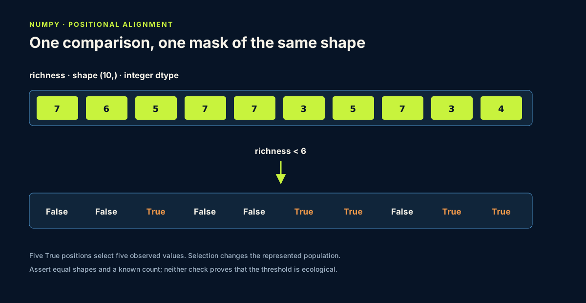
In Lesson 5, a loop visited one plot at a time. NumPy expresses the comparison at the collection level:

below_six = richness < 6

NumPy still performs work for every element, but the iteration is implemented inside the library. The array expression is concise, often faster and easier to compare with the mathematical method. It also reduces the chance that one item receives different code accidentally.

Vectorisation is appropriate only when the elements are comparable. Combining species counts, heights and dates in one numerical array would destroy meaning even if Python accepted the values.

Prove equivalence with the Lesson 5 loop

Use the same first-six richness values from Lesson 5: 7, 6, 5, 7, 7, 3. The loop produced total 35, used-value count 6, mean 35 / 6 and two values below 6. Create a NumPy array and assert that its sum, size, mean and below-six count agree with those recorded results.

This is a controlled implementation comparison. Agreement increases confidence that vectorisation preserved the calculation; it does not independently validate the records or threshold.

Check your understandingWhy must a Boolean mask align with its source array?

Choose one answer

Each True or False selects the value at the same positionMasks use field namesAlignment changes the units

Check answer

5. Select values with a Boolean mask

review_values = richness[below_six]

print(review_values)
print(review_values.mean())

Square brackets now mean selection. The Boolean mask keeps values where the corresponding position is True. This is positional alignment: the mask must have the same shape as the array it filters.

The selected mean answers “What is the mean among values below the instructional threshold?” It must not be compared casually with the full mean because the subset was created by the value being summarised.

Scientific note: filtering changes the population represented by a result. Every figure and statistic should make the selection rule visible.

6. Missing values change numerical behaviour

NumPy can represent a missing numerical value with np.nan, which stands for “not a number.” Introducing np.nan usually makes an integer array become floating point because ordinary integer storage has no nan representation.

biomass = np.array([311.33, 228.44, np.nan, 284.78])

print(biomass.dtype)
print(np.mean(biomass))
print(np.nanmean(biomass))

The ordinary mean returns nan because missingness propagates. np.nanmean excludes missing values, but that exclusion is a scientific decision. Report both the number of available observations and the policy used. In the full dataset, 59 of 120 AGB cells are empty; missingness is substantial, not incidental.

Count the evidence explicitly:

missing_mask = np.isnan(biomass)
missing_count = missing_mask.sum()
available_count = biomass.size - missing_count

print("Available:", available_count)
print("Missing:", missing_count)
print("Available-value mean:", np.nanmean(biomass))

Do not test missing numerical values with biomass == np.nan; np.nan does not compare equal to itself. Use np.isnan for this numerical array. The full pandas table will use pd.isna() in Lesson 9 because it must handle more than one missing representation.

7. From a column to a grid

The richness array has one dimension: one sequence of values. Remote-sensing rasters are commonly represented by two-dimensional arrays whose first dimension contains rows and whose second dimension contains columns. This small synthetic reflectance grid is not part of the published field table and is not yet a georeferenced raster. It introduces only the array structure you will use in Module 2.

Before running, predict the shape, the number of dimensions, the upper-left value, the first row and the first column:

reflectance_grid = np.array([
    [0.18, 0.21, 0.24, 0.20],
    [0.25, 0.29, 0.31, 0.27],
    [0.22, 0.26, 0.28, 0.23],
])

print("Shape:", reflectance_grid.shape)
print("Dimensions:", reflectance_grid.ndim)
print("Upper-left value:", reflectance_grid[0, 0])
print("First row:", reflectance_grid[0, :])
print("First column:", reflectance_grid[:, 0])

Expected structural results are shape (3, 4) and ndim equal to 2: three rows by four columns. In array[row, column], reflectance_grid[0, 0] selects one value. The colon means “all positions” along that dimension, so [0, :] selects every column in the first row and [:, 0] selects the first column across every row.

The first displayed row is not automatically the northern edge of a real image, and columns are not automatically eastings. Array position gains spatial meaning only through raster metadata and a documented orientation. Preserve this distinction when describing the synthetic grid.

Bridge to Module 2: a numerical grid does not become geospatial merely because it has rows and columns. A raster also needs spatial metadata connecting those positions to an extent, resolution and coordinate reference system.

Learner action

Run the grid cell, compare each output with your prediction and change only the value at row 1, column 2. Explain why Python uses zero-based positions and why the array shape alone cannot tell you where this grid is located on Earth.

8. Common mistakes and recovery

Mixing incompatible meanings

Recognition: an array contains richness counts, moisture values and heights because all happen to be numeric. Fix: create arrays by documented variable and confirm units and meaning before calculation.

Confusing shape with value count

Recognition: (10,) is read as ten rows and an unknown number of columns. Fix: interpret it as one axis of length ten; use .ndim and .size when unsure.

Expecting a Python list comparison to behave like NumPy

Recognition: python_list < 6 raises TypeError. Fix: convert an appropriate homogeneous numerical list to an array, then inspect its shape and dtype.

Ignoring mask alignment

Recognition: selection fails because the mask has a different length, or a mask from another variable is reused without confirmed alignment. Fix: build the mask from the array being selected and check both shapes.

Using nanmean without reporting missingness

Recognition: a plausible mean hides that nearly half the biomass records were absent. Fix: count available and missing observations and state the exclusion policy with the result.

9. Guided practice, independent challenge and portfolio artifact

Guided practice — a second published field

Create a NumPy array from the first six Height_median values: 27, 29, 23, 35, 29, 29.

1. Predict shape and dtype.
2. Calculate minimum, maximum and mean.
3. Create a mask for values at least 29.
4. Count and display the selected values.
5. Describe them as values from the first six rows; do not attach an unsupported unit.

Independent challenge — moisture sequence

Use the first six Moisture_mean values: 14.33, 13.23, 17.03, 24.53, 25.87, 17.47.

• Create and inspect an array.
• Calculate its mean and median.
• Create one clearly labelled instructional threshold mask.
• Report the selected count and values.
• Explain why this six-row subset and undocumented unit limit the scientific claim.

Professional QA decision

Classify the numerical result as:

• ready for the current subset when provenance, scope, shape, dtype, mask alignment, missingness counts and known-answer checks agree;
• review when a structural expectation or loop-equivalence check fails;
• stop when values of incompatible meaning or undocumented positional alignment have been combined.

For the synthetic grid, report array structure verified; spatial meaning not assigned. That is the scientifically accurate handover state before Module 2 supplies geospatial metadata.

Answer in private notes:

1. What does array shape tell you that a printed list may not make obvious?
2. Why does a Boolean mask need positional alignment?
3. What decision is hidden inside np.nanmean?
4. When is a clear loop preferable to a compact vectorised expression?
5. Why does a verified (3, 4) shape not establish the grid's location or orientation?

Submission

• Notebook: verified richness, height and moisture array sections with predictions, outputs and interpretations.
• Screenshot: the moisture mask and its selected output.
• Written answer: 200–280 words explaining vectorisation, shape, dtype, missingness policy and the limits of the subset.

Portfolio artifact

Artifact 07 — Verified numerical-array analysis

This seventh checkpoint in Portfolio Project 1 — Vegetation Data Explorer demonstrates that you can move from small Python collections to structured scientific arrays while preserving provenance, denominators, positional alignment and interpretation limits.

From the Field — arrays need meaning

An array axis must identify its entity: individual leaves, species summaries or plots are not interchangeable rows. Record axis, unit and support before computing with CCI, leaf area or cover. Trace leaf measurements into plot CWM.