Missing Values, Types and Data Quality

Learning pathway

You already know

Lesson 6 documented a deliberately narrow scalar function. Lesson 8 identified the exact published file, parser choices and expected table structure, then accepted it only for this quality audit.

In this lesson

You will separate observed quality evidence from scientific rules and actions. You will upgrade the earlier function for pandas representations, profile missingness by denominator and sampling group, inspect conversion loss and preserve every source value beside derived flags.

Why this comes now

Filtering or summarising before profiling can silently redefine the analysis population. Quality decisions must therefore be attached to named fields, documented evidence and a specific future question before rows are selected.

You will use this later

Lesson 10 creates analysis populations from this evidence, Lesson 11 validates derived-table joins and Lesson 12 communicates unresolved limitations. Module 2 applies the same observe–rule–action separation to geometry, raster and UAV QA.

1. Profile the table before deciding how to clean it

Learning outcome

By the end of this lesson, you will be able to create a reproducible data-quality profile for selected columns, distinguish missing, invalid and inconsistent values, and document a field-specific response without overwriting the raw data. You will add a quality report to the Vegetation Data Explorer.

Prerequisites: Complete Lessons 1–8 and keep the published CSV in the project data folder. Allow 90–110 minutes.

Why this matters

Missingness can reflect sampling design rather than failure. A negative value can be impossible for biomass but valid for an isotope measurement. A numeric-looking column can become text because one cell contains a note. Treating all these cases with one “clean data” command destroys evidence.

Professional quality control separates three stages: observe the current state, define a rule with scientific justification, and record the response. The original source remains unchanged so every transformation can be reviewed.

Scientific context

The published table has no missing Sp_richness or CCI_CWM values, but 59 of 120 AGB cells are empty. N_AGB_Sample is empty in the same number of rows. This pattern is large enough to influence any biomass summary and may reflect how above-ground biomass samples were collected. The CSV alone does not establish the reason.

Core idea: a quality profile describes what is present; a cleaning decision states what to do and why. Do not confuse the two.

Learner action

Add ## Lesson 9 — Data quality profile. Write three separate definitions in your own words: missing value, invalid value and inconsistent representation.

Separate four quality dimensions

Dimension	Question	Example evidence	Why it stays separate
completeness	is a value present?	AGB missing count and percentage	absence is not the same as invalidity
conformance	is the representation usable under the contract?	numeric, text, Boolean or missing scalar	a valid type does not validate the measurement
consistency	do related fields agree structurally?	Height_max >= Height_median	a conflict needs review, not an invented correction
uniqueness/identity	is each required entity identifiable once?	complete, non-duplicated SampleID	unique IDs do not validate other fields

The profile reports evidence in each dimension. An action comes later and must name the question for which it is appropriate.

2. Count missingness explicitly

Worked example

Predict which field will have the largest missing percentage:

quality_fields = [
    "SampleID",
    "site",
    "Sp_richness",
    "CCI_CWM",
    "AGB",
    "N_AGB_Sample",
]

quality_profile = pd.DataFrame({
    "dtype": meadows[quality_fields].dtypes.astype(str),
    "missing_n": meadows[quality_fields].isna().sum(),
    "unique_n": meadows[quality_fields].nunique(dropna=True),
})
quality_profile["missing_pct"] = 100 * quality_profile["missing_n"] / len(meadows)
print(quality_profile.round({"missing_pct": 1}))

AGB and N_AGB_Sample should each report 59 missing values, or 49.2% when rounded to one decimal place.

Code walkthrough

1. quality_fields makes the audit scope visible.
2. meadows[quality_fields] selects those columns without changing the source table.
3. .dtypes.astype(str) records pandas storage types as readable labels.
4. .isna() produces a Boolean table; .sum() counts True values per column.
5. .nunique(dropna=True) counts distinct present values.
6. The percentage uses the full 120-row table as its denominator.
7. .round(...) changes display precision, not the underlying counts.

Check your understandingWhat should accompany a missing-value percentage?

Choose one answer

The count and denominatorA claim that missing equals zeroAutomatic row deletion

Check answer

3. Interpret pandas types cautiously

pandas often uses:

• object or string for text labels;
• int64 for complete whole-number columns;
• float64 for decimal values and for whole-number fields that also contain NaN;
• datetime64[ns] for parsed dates;
• bool for Boolean values.

A dtype is a storage description. It does not tell you whether CCI_CWM and LA_CWM share a unit, whether a community code is documented or whether a measured value is plausible.

Use pd.to_numeric on a copy when a field should be numeric but loads as text:

candidate = meadows["AGB"].copy()
converted = pd.to_numeric(candidate, errors="coerce")
new_missing = converted.isna() & candidate.notna()

print("Unparseable present values:", new_missing.sum())

errors="coerce" changes unparseable values to NaN. That is useful for detection but dangerous as silent cleaning. The new_missing mask identifies values that conversion would erase, so they can be inspected first.

Print candidate[new_missing] with SampleID before accepting any conversion. Preserve the original series and count present values before and after conversion. A zero new_missing count supports representation compatibility for the current file; it does not validate units or plausibility.

Check your understandingWhat risk does `errors="coerce"` create?

Choose one answer

Unparseable present text can become missing silentlyEvery number becomes a dateIt validates the measurement

Check answer

4. Upgrade an earlier function as the data become more realistic

In Lesson 6, classify_biomass() handled None, the missing-value representation you had learned at that point. Its documented boundary was intentionally narrow. After meeting NumPy and pandas, you now know that a table value may also arrive as np.nan. Because np.nan is a floating-point value, the earlier function could incorrectly classify it as "recorded".

Do not erase the earlier version or describe it as a secret mistake. Preserve it as evidence of how the specification evolved, then add this pandas-aware version beneath it:

def classify_biomass_pandas(value):
    """Classify one scalar AGB value from a pandas workflow."""
    if isinstance(value, (bool, np.bool_)):
        return "invalid Boolean"
    if pd.isna(value):
        return "missing"
    if not isinstance(value, (int, float, np.integer, np.floating)):
        return "invalid type"
    if value < 0:
        return "invalid negative"
    return "recorded"

test_values = [None, np.nan, 311.33, -1, "311.33", True]
for test_value in test_values:
    print(repr(test_value), classify_biomass_pandas(test_value))

Predict all six results before running. Expected output:

None missing
nan missing
311.33 recorded
-1 invalid negative
'311.33' invalid type
True invalid Boolean

pd.isna() recognises both None and np.nan as missing scalar values. The Boolean check still comes first because Python Booleans belong to the integer type hierarchy; a quality flag must not become a biomass measurement. NumPy numeric scalar types are accepted because pandas columns can supply them. A numeric-looking string remains text until provenance and parsing rules justify conversion.

Make the six expectations executable:

assert classify_biomass_pandas(None) == "missing"
assert classify_biomass_pandas(np.nan) == "missing"
assert classify_biomass_pandas(311.33) == "recorded"
assert classify_biomass_pandas(-1) == "invalid negative"
assert classify_biomass_pandas("311.33") == "invalid type"
assert classify_biomass_pandas(True) == "invalid Boolean"

This function contract accepts one scalar value at a time. Passing a complete Series would make pd.isna(value) return a Boolean Series rather than one decision, so table-wide checks should use vectorised masks directly.

Learner action — compare specifications, not only outputs

Create a six-row Markdown test table with columns input, Lesson 6 expectation, Lesson 9 expectation and reason. Run each value through both function versions. Identify the np.nan case whose result changes and explain why the new result reflects a more realistic data representation rather than an arbitrary code correction.

This is iterative scientific programming: new data structures expose a limitation, the function contract is revised explicitly, and all known cases are rerun. The history matters because future reviewers need to know which assumptions changed and why.

5. Build field-specific checks

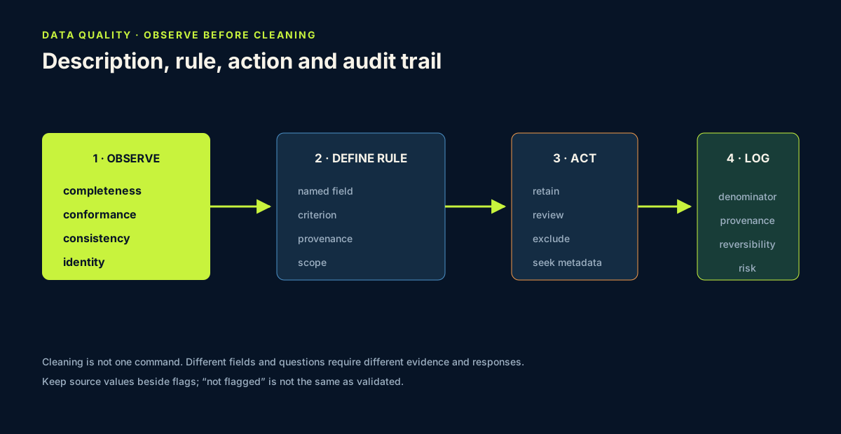
Use rules appropriate to each field:

• Identity: SampleID should be present and unique for this table.
• Category consistency: site and community labels should be inspected for unexpected spelling, capitalisation and surrounding whitespace.
• Completeness: missingness should be counted overall and by relevant sampling groups.
• Range validity: a range must come from field meaning or protocol; do not apply one generic range to every numeric column.
• Relational consistency: Height_max would normally be expected to be at least Height_median; a failure should be flagged for review, not automatically “fixed.”
• Temporal consistency: parsed dates should fall inside the documented collection period.

checks = pd.DataFrame(index=meadows.index)
checks["duplicate_id"] = meadows["SampleID"].duplicated(keep=False)
checks["height_order"] = meadows["Height_max"] < meadows["Height_median"]
checks["negative_agb"] = meadows["AGB"].notna() & (meadows["AGB"] < 0)
checks["missing_agb"] = meadows["AGB"].isna()

print(checks.sum())

The checks table stores review evidence separately from the measurements. A False result means the record did not trigger that specific rule; it does not certify the complete row.

Check your understandingWhy should range checks be field-specific?

Choose one answer

Different variables have different meanings and valid domainsAll numeric fields share one rangepandas requires one rule per table

Check answer

6. Ask whether missingness follows the sampling structure

Overall missingness is only the beginning. Compare available and missing biomass counts by site and plant community:

agb_coverage = (
    meadows.assign(AGB_available=meadows["AGB"].notna())
    .groupby(["site", "plantcommunity"], observed=True)["AGB_available"]
    .agg(available_n="sum", total_n="size")
)
agb_coverage["available_pct"] = 100 * agb_coverage["available_n"] / agb_coverage["total_n"]
print(agb_coverage)

This does not explain the missingness, but it reveals whether availability is evenly distributed among sampled groups. If missingness is related to sampling design, dropping incomplete rows could change which sites or communities dominate the analysis.

The identical overall missing count for AGB and N_AGB_Sample does not prove that the same rows are missing. Compare their Boolean missingness masks and count disagreements. Report the observed pattern, but do not label a statistical missingness mechanism or sampling cause without appropriate design evidence.

7. Common mistakes and recovery

Calling empty cells zero

Recognition: missing biomass is filled with 0 before its cause or analysis purpose is considered. Fix: retain NaN, quantify missingness and choose any imputation only with a defensible model and sensitivity analysis.

Running dropna() on the entire table

Recognition: rows are removed because of fields irrelevant to the current question. Fix: define the analysis variables first and assess missingness only for that explicit subset.

Applying one range to every numeric field

Recognition: valid negative isotope values are flagged merely because biomass cannot be negative. Fix: attach rules to named fields and documented meanings.

Treating object as proof of bad data

Recognition: categorical labels are converted or deleted simply because dtype is object. Fix: inspect values and use an intentional string or categorical representation.

Correcting without an audit trail

Recognition: source values are overwritten and the notebook cannot show what changed. Fix: preserve raw columns, create flags or derived columns, and record rationale.

Assuming absence of flags means validity

Recognition: a short checks table is called “validated data.” Fix: describe the scope of the checks and the risks not evaluated.

8. Guided practice — create a quality decision log

For SampleID, Date, site, Sp_richness, Height_median, Height_max and AGB:

1. report dtype, missing count and unique count;
2. define one check that is justified by structure or field relationship;
3. calculate how many rows trigger it;
4. select and display triggered rows with their identifiers;
5. write the action: retain, review, exclude for a named analysis, or seek metadata;
6. record what evidence would be required before correction.

Use a Markdown decision log with columns field, observation, rule, triggered, action, justification.

Add denominator, rule provenance, reversibility and unresolved risk columns. A count of triggered rows without its denominator is incomplete, and an action that cannot be reversed requires stronger evidence than a derived review flag.

9. Independent challenge, reflection and portfolio artifact

Choose one future question involving Sp_richness and one involving AGB.

• Define the minimum columns required for each question.
• Create separate completeness profiles.
• Compare group coverage by site.
• Explain how the analysis population changes when AGB is required.
• Produce a quality_flags table containing SampleID and your documented Boolean checks.
• Do not delete rows or overwrite measurements.

Professional data-readiness decision

Make one decision for each future question, not one global “clean data” label:

• conditionally ready when required fields, completeness, conformance, consistency checks, population impact and unresolved risks are documented;
• review when a rule lacks provenance or group coverage may materially change interpretation;
• stop when identity, representation loss or required-field evidence is unresolved.

State which derived flags and source columns must travel into Lesson 10. A dataset can be conditionally ready for a richness summary while unready for a biomass question because the required evidence and analysis populations differ.

Scientific interpretation

The quality report establishes that biomass availability differs from richness availability and that specific structural checks can be reproduced. It does not identify why biomass is absent or guarantee the ecological validity of present measurements. Those questions require sampling metadata and subject-matter review.

Answer in private notes:

1. Why can missingness be scientifically informative?
2. What does coercion risk hiding?
3. Why should a validity rule name its field?
4. What difference is there between “not flagged” and “validated”?
5. Why can equal missing counts in two fields hide different missing rows?

Submission

• Notebook: quality profile, checks table, group coverage analysis and decision log.
• Screenshot: the quality profile and at least one set of triggered-row evidence.
• Written answer: 250–350 words explaining missingness pattern, field-specific rules, chosen actions and unresolved metadata questions.

Portfolio artifact

Artifact 09 — Auditable ecological data-quality report

This ninth checkpoint in Portfolio Project 1 — Vegetation Data Explorer demonstrates that you can diagnose a real scientific table without erasing uncertainty, disguising cleaning decisions or labelling the complete dataset “clean” for every question.

From the Field — missing traits are not zero

The CCI and leaf-area tables are a real missing-data case: only species summaries with at least five measurements are used, and their represented share of species-only cover must be audited. An absent trait value means unavailable evidence, not a measured zero. Review the documented aggregation and limitations.