Filter, Group and Summarise

Learning pathway

You already know

Lesson 9 produced question-specific readiness decisions, source-preserving flags and group-coverage evidence. Those decisions now determine which rows and fields may enter each summary.

In this lesson

You will write an analysis specification, create and audit its population mask, summarise defined groups with denominators and spread, and test whether grouped results reconcile with the selected rows.

Why this comes now

A statistically correct aggregation can answer the wrong question when the population or grouping structure is hidden. Analysis starts only after intake and quality evidence establish what can be compared.

You will use this later

Lesson 11 joins and reshapes these audited summaries, and Lesson 12 uses them in a claim–evidence chain. Later EO modules apply the same logic to pixels, dates, validation samples and model-error groups.

1. Match the table operation to the scientific question

Learning outcome

By the end of this lesson, you will be able to define an analysis population with a Boolean filter, group rows by a documented category, and report sample size with appropriate descriptive statistics. You will explain why a group difference is descriptive rather than automatically causal.

Prerequisites: Complete Lessons 1–9 and retain the meadows DataFrame and quality report. Allow 90–110 minutes.

Why this matters

“What is the average?” is incomplete. Average of which variable, among which observations, grouped by what, with how many measurements and under which missing-value rule? Filtering and grouping convert a broad table into an explicit analytical comparison.

Remote sensing analyses rely on the same pattern: select cloud-free observations, group pixels by land-cover class, summarise a time series by month or compare model error by site. If the analysis population is hidden, the result cannot be interpreted or reproduced.

Scientific context

The table contains four sites with unequal row counts: Kudani 40, Keemu 30, Koera 30 and Saardu 20. The four plant-community codes also occur in different combinations across sites. A site-level mean therefore combines sampling composition as well as vegetation measurements.

Core idea: filter defines which rows answer the question; group defines which rows are compared; summary describes each group and must retain its denominator.

Learner action

Add ## Lesson 10 — Filter, group and summarise. Write one complete analytical question in this form: “Among [explicit rows], how does [named variable] differ by [group]?”

Write the analysis specification

Element	Required statement	Review question
unit represented by one row	one published quadrat record	does the design support treating records as independent?
analysis population	explicit inclusion and missingness criteria	how many source rows are included and excluded?
response	exact field, meaning and unresolved unit status	are values comparable under one summary?
grouping	exact categorical field and observed levels	is group composition confounded with another field?
estimands	n, mean, median and standard deviation	what does each statistic describe?
interpretation scope	sampled records in this table	which causal or regional claims remain unsupported?

n_plots counts distinct sample identifiers here. Do not call this a count of independent observations unless the sampling design supports independence.

2. Build a Boolean filter you can count and inspect

Suppose the immediate question is: “Among Saardu quadrats with recorded species richness, what values were observed?”

is_saardu = meadows["site"] == "Saardu"
has_richness = meadows["Sp_richness"].notna()
analysis_mask = is_saardu & has_richness

saardu_richness = meadows.loc[
    analysis_mask,
    ["SampleID", "plantcommunity", "Sp_richness"],
].copy()

print("Selected rows:", analysis_mask.sum())
print(saardu_richness.head())

& combines two element-by-element Boolean conditions. Parenthesise comparisons when writing them directly. .loc[row_condition, columns] makes row and column selection visible. .copy() creates an independent analysis table so later derived columns do not ambiguously modify a view.

Always inspect selected row count and identifiers. A filter that returns zero or every row may still be syntactically correct but inconsistent with the intended question.

Check your understandingWhen should the analysis-population filter be applied?

Choose one answer

Before grouping and summarisingOnly to the displayed resultAfter writing the conclusion

Check answer

3. Group rows and retain the evidence behind a mean

Worked example

Predict which site has the highest mean Sp_richness, then run:

analysis = meadows.loc[
    meadows["Sp_richness"].notna(),
    ["SampleID", "site", "plantcommunity", "Sp_richness"],
].copy()

site_summary = (
    analysis.groupby("site", observed=True)
    .agg(
        n_plots=("SampleID", "nunique"),
        richness_mean=("Sp_richness", "mean"),
        richness_median=("Sp_richness", "median"),
        richness_sd=("Sp_richness", "std"),
    )
    .sort_values("richness_mean", ascending=False)
)

print(site_summary.round(2))

The site means should be approximately Keemu 13.10, Koera 12.07, Saardu 8.45 and Kudani 5.05. These are reproducible descriptive values from the current table.

Code walkthrough

1. The analysis table includes only the identifier, grouping fields and response variable.
2. The explicit non-missing filter defines the analysis population; no richness rows are actually missing, but the policy remains visible.
3. groupby("site") partitions rows by exact site label.
4. .agg(...) calculates several named outputs for every group.
5. nunique counts distinct sample identifiers rather than assuming row count equals sample count.
6. Mean describes arithmetic centre; median is resistant to extreme values; standard deviation describes spread around the mean.
7. Sorting changes presentation order, not the group calculations.
8. Rounding is applied only for display.

Standard deviation describes variation among observed values within each group. It is not a confidence interval, standard error or direct measure of uncertainty in the group mean.

Reconcile the grouped result with its population

assert site_summary["n_plots"].sum() == analysis["SampleID"].nunique()

weighted_mean = (
    site_summary["richness_mean"] * site_summary["n_plots"]
).sum() / site_summary["n_plots"].sum()
assert np.isclose(weighted_mean, analysis["Sp_richness"].mean())

The first check detects lost or duplicated identifiers across mutually exclusive site groups. The second shows why an unweighted mean of four site means would not reproduce the plot-level mean when group sizes differ.

Check your understandingWhy report `n` beside a group mean?

Choose one answer

It shows how many observations support the summaryIt makes every group balancedIt proves causality

Check answer

4. Read summaries as distributions, not rankings alone

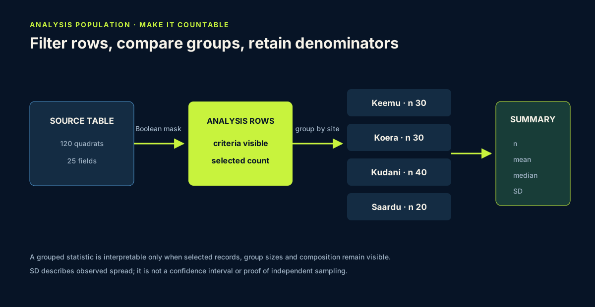
A professional summary should answer:

• how many records and distinct sample identifiers contributed?
• what evidence supports or limits independence?
• which measure of centre was used?
• how variable were observations within the group?
• were missing values excluded, and how many?
• is the grouping factor confounded with another sampled factor?

The largest mean should not automatically become “the best site.” Species richness is one ecological property, and observed differences may reflect plant-community composition, location, sampling conditions or other factors not modelled here.

Check your understandingWhat is justified by a higher mean richness at one sampled site?

Choose one answer

A descriptive difference in this tableProof that site caused higher richnessGuaranteed regional ranking

Check answer

5. Compare two grouping structures

Create a community summary with the same outputs:

community_summary = (
    analysis.groupby("plantcommunity", observed=True)
    .agg(
        n_plots=("SampleID", "nunique"),
        richness_mean=("Sp_richness", "mean"),
        richness_median=("Sp_richness", "median"),
    )
    .sort_values("richness_mean", ascending=False)
)
print(community_summary.round(2))

The four community-code means are approximately TG 15.93, US 11.70, LS 5.60 and OP 4.30. Preserve the codes exactly; do not invent expanded names. Compare site and community summaries and notice that these factors are not distributed in a complete balanced grid.

Create a site-by-community count table before interpreting either grouping. Empty or sparse combinations show where a site mean represents a different community composition. Stratified description can expose this pattern, but it does not by itself remove confounding or establish a causal site effect.

6. Common mistakes and recovery

Filtering after calculating the summary

Recognition: the statistic includes rows outside the question, then only the display is filtered. Fix: define and inspect the analysis population before grouping.

Reporting a mean without n

Recognition: groups with 20 and 40 observations appear equally supported. Fix: report count beside centre and spread.

Taking an unweighted mean of group means

Recognition: four site means are averaged as if each represented the same number of plots. Fix: calculate the overall mean from rows, or use an explicitly justified weighting method.

Treating missing as zero

Recognition: biomass summaries become artificially low. Fix: define the non-missing analysis population and report availability for every group.

Hiding a filter in a long expression

Recognition: the notebook cannot easily display how many rows each criterion selected. Fix: name intermediate Boolean masks and audit their counts.

Making a causal statement from grouped descriptions

Recognition: a higher group mean is attributed to site conditions without design or modelling evidence. Fix: use “observed in this sample” language and list plausible confounding factors.

7. Guided practice — biomass coverage and summary

Investigate AGB by site:

1. create a Boolean mask for present biomass;
2. count available and missing rows by site;
3. calculate n, mean, median and standard deviation only among present values;
4. combine coverage and summary in one readable table;
5. compare the analysis sample size with all 120 quadrats;
6. explain why the highest observed mean should be interpreted cautiously.

The present-value site means should be approximately Saardu 201.32, Koera 108.15, Keemu 102.62 and Kudani 78.63. Use these values only to verify your code; report output calculated by your notebook.

8. Independent challenge, reflection and portfolio artifact

Choose either Height_median or CCI_CWM as the response.

• Write one explicit analytical question.
• Define and count the analysis population.
• Produce comparable summaries by site and by plant-community code.
• Include n, mean, median and standard deviation.
• Identify the largest difference between mean and median.
• Select the underlying rows for that group and inspect whether unusual values may contribute.
• Write a cautious 150-word interpretation without causal claims.

Professional analysis decision

Classify the result as:

• ready for descriptive handover when the question, population, denominators, missingness policy, reconciliation checks and design limits are explicit;
• review when group composition, sparse cells or unusual values materially affect interpretation;
• stop when the required field was not conditionally ready in Lesson 9 or the selected rows cannot be reconstructed.

Record the exact input flags and mask used. A summary table without a reproducible route back to its records is not a complete portfolio artifact.

Answer in private notes:

1. What exact rows does your result represent?
2. Why is n part of the scientific result?
3. When might median communicate centre better than mean?
4. Which design feature prevents a simple site comparison from isolating cause?
5. Why does within-group standard deviation not quantify uncertainty in the mean by itself?

Submission

• Notebook: named filters, site and community summaries, biomass guided practice and independent interpretation.
• Screenshot: a complete summary table including n, centre and spread.
• Written answer: 250–350 words stating the question, population, grouping, missing-value policy, result and interpretation limits.

Portfolio artifact

Artifact 10 — Reproducible grouped vegetation summary

This tenth checkpoint in Portfolio Project 1 — Vegetation Data Explorer demonstrates that you can move from a research question to an explicit analytical population, reconcile grouped results with source records and communicate an appropriately qualified comparison.

Species Atlas activity

Summarise occurrence as occupied plots divided by sampled plots, then summarise positive cover only among plots with numeric cover. Report the denominator: prevalence and abundance answer different questions. Compare observed habitat frequencies in the Species Atlas.