What Makes Data Geospatial?

1. Begin with spatial evidence, not a map

Learning outcome

By the end of this lesson, you will be able to decide whether a dataset is tabular, vector, raster, or spatial with incomplete reference metadata. You will identify the evidence for location, geometry, grid structure and spatial reference, and create the first component of your Module 2 portfolio: spatial_data_inventory.ipynb.

Prerequisites: Module 1 or equivalent confidence with Jupyter, Python dictionaries, lists, loops and pandas-style tables. No GIS software experience is assumed. Allow 60–80 minutes.

Why this matters

Many serious spatial errors begin before analysis. A file opens, coordinates look numerical, and a map appears. The result feels geospatial, but the evidence connecting the values to Earth may be missing or misunderstood.

A professional remote-sensing scientist does not ask only, “Can I plot this?” The stronger question is:

What evidence connects every observation to a location, spatial representation and reference system?

This question determines whether field measurements can be joined to imagery, whether an area is meaningful, and whether a result can be reproduced by another analyst. A polished map cannot repair missing spatial metadata.

Scientific context

You are continuing the Baltic coastal-meadow research story from Module 1. The published plant-traits table contains sample identifiers, site labels and ecological measurements. It does not publish plot coordinate columns. A site label is useful context, but it is not a point geometry and does not reveal the precise location of a quadrat.

The research group now gives you four data handover cards:

Asset	Evidence supplied	Important limitation
baltic_plant_traits.csv	rows, fields, SampleID, site labels	no coordinate or geometry fields
training_transect.geojson	ordered coordinate pairs and LineString geometry	location depends on the GeoJSON spatial convention
uav_reflectance_demo.tif	rows, columns, transform, bounds and CRS	band meaning and acquisition metadata still require verification
unverified_plot_xy.csv	numeric x and y fields	CRS, axis meaning and units are absent

Only the first card represents the published Zenodo table. The other three are instructional assets for learning spatial reasoning; they are not claimed to contain published Baltic plot locations.

Learner action

Download and open the UAV and Satellite Analysis Pipeline starter notebook. Add a Markdown heading ## Lesson 2.1 — What makes data geospatial?. Under it, write your initial classification of the four assets. Do not search by file extension yet. Use only the evidence in the table.

2. Location is necessary, but it is not sufficient

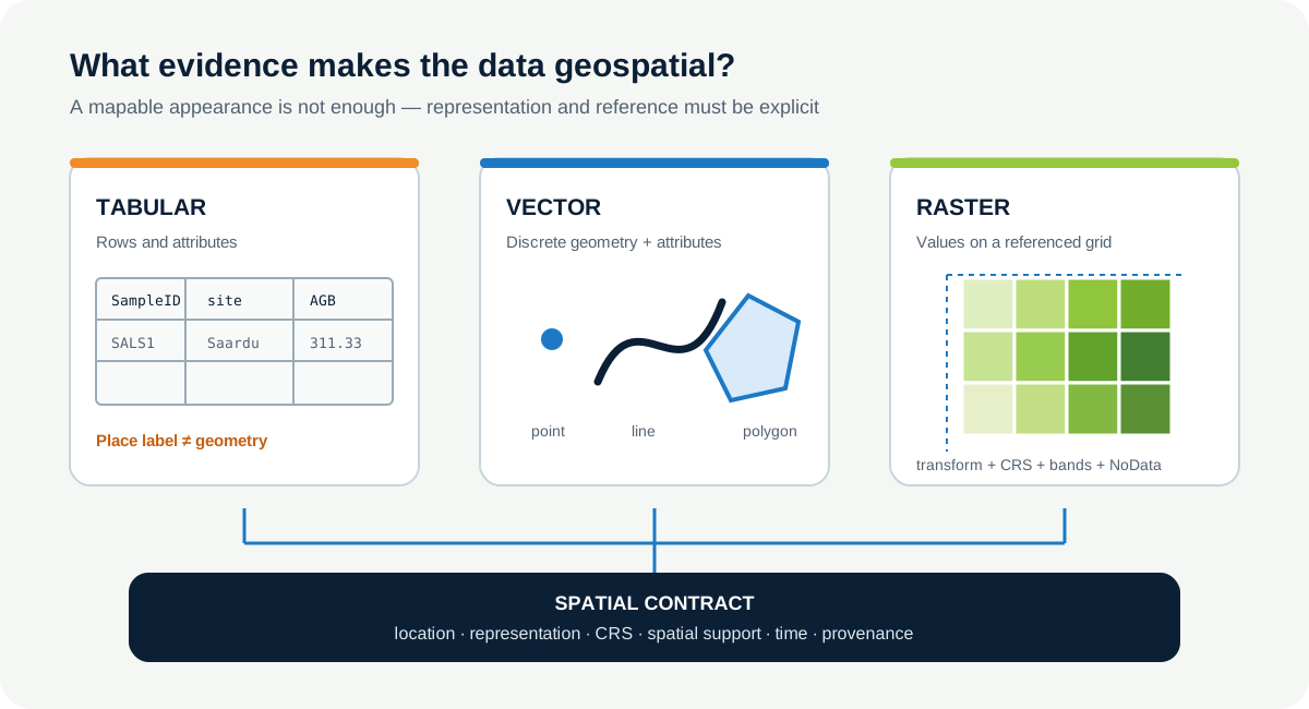
Data become geospatial when their values can be interpreted in relation to location on Earth. That connection can be represented in several ways:

• explicit coordinates, such as longitude and latitude;
• geometry, such as a point, line or polygon;
• a referenced grid, where row and column positions are connected to Earth coordinates by a transform;
• a documented relationship to another spatial dataset, such as a stable site identifier joined to a verified site boundary.

An ordinary table may contain place-related text without containing geometry. site = "Saardu" tells you which site label is attached to a record, but it does not identify a unique point, boundary or coordinate reference. The table can later participate in a spatial workflow through a documented join. It should not be silently converted into invented point locations.

A coordinate pair also needs interpretation. The values (24.75, 59.45) could plausibly be longitude and latitude in decimal degrees. The values (542000, 6584000) could plausibly be eastings and northings in metres. Plausibility is not proof. You still need axis order, units, coordinate reference system and provenance.

Check your understandingThe Baltic field table contains site names and sample identifiers but no coordinates or geometry. What can you conclude?

Choose one answer

It is tabular data with location-related attributes, but it cannot yet be mapped as featuresEvery row is automatically a point featureThe site name proves an EPSG code

Check answer

3. Vector data represent discrete geometries

The vector model represents spatial objects with coordinate-based geometry. Three basic geometry types provide the foundation:

• a point represents a location with no area at the selected model scale, such as a verified sampling position;
• a line represents an ordered path or network, such as a survey transect or drainage channel;
• a polygon represents an enclosed area, such as a management zone or meadow boundary.

Geometry is a model, not the phenomenon itself. A plot point may represent the centre of a one-square-metre quadrat, but the point has no area. If the analysis needs the sampled footprint, that support must be represented or documented separately. A coastline stored as a line is also a scale-dependent approximation of a changing boundary.

Vector features commonly combine one geometry with attributes in each row. This resembles the pandas tables used in Module 1, with an additional geometry column and a spatial reference. Later lessons will use GeoPandas to work with this structure. For now, the important question is what one feature represents.

4. Raster data represent a referenced grid

The raster model divides an extent into cells arranged by row and column. Each cell stores a value for one band: reflectance, elevation, temperature, land-cover class or another variable. A multiband raster stores several aligned grids.

An array of numbers is not automatically a geospatial raster. It becomes spatially interpretable when metadata connect array positions to Earth locations. That spatial contract normally includes:

• number of rows and columns;
• pixel size and orientation;
• an affine transform connecting grid positions to coordinates;
• a coordinate reference system;
• spatial extent;
• NoData meaning;
• band definitions, units and acquisition information.

The 2-D NumPy bridge in Module 1 taught array[row, column]. Raster science adds the metadata that explain where that cell is, what area it supports and what its value means.

Check your understandingWhich distinction best separates vector and raster representations?

Choose one answer

Vector stores discrete geometries; raster stores values on a referenced gridVector is always accurate; raster is always approximateVector contains attributes; raster never does

Check answer

5. Spatial reference makes coordinates interpretable

A coordinate reference system, or CRS, defines how coordinate values relate to Earth. It describes matters such as the datum, coordinate axes, units and map projection. Lesson 2.2 develops these ideas carefully.

For this lesson, use one strict rule:

Coordinates without a verified CRS are spatial intent, not analysis-ready location.

Do not guess a CRS by trying several options until the layer lands somewhere familiar. Many incorrect CRSs can produce superficially plausible maps. Record the values as received, quarantine the asset from spatial analysis and investigate its source, export settings, accompanying metadata and data producer.

GeoJSON requires special care. The current GeoJSON standard, RFC 7946, defines positions using WGS 84 longitude and latitude in decimal degrees, with longitude first. Older files and software may contain non-standard conventions. Check the file history and the software that produced it instead of relying only on the extension.

Check your understandingA table contains x = 650000 and y = 6430000 but no CRS. What is the defensible next action?

Choose one answer

Quarantine it as spatial data with unverified CRS metadata and investigate provenanceAssume longitude and latitude because there are two numbersPlot it and keep whichever map looks plausible

Check answer

Accuracy, precision, resolution, uncertainty and error

These words answer different questions. Keep them separate when accepting spatial data:

Term	Practical meaning	Coastal-meadow example
accuracy	closeness to a trusted reference or true value	how close a mapped plot position is to independently surveyed control
precision	repeatability or numerical/detail consistency	repeated GNSS fixes cluster tightly, even if the cluster is displaced
resolution	smallest sampling interval or detail represented	a UAV orthomosaic is delivered with 5 cm pixels
uncertainty	quantified or described limits on what is known	horizontal position is reported with a 95% uncertainty interval
error	difference from a reference value when that reference is available	mapped checkpoint minus surveyed checkpoint position

Fine resolution does not prove high accuracy. High precision does not prevent systematic error. Uncertainty is not carelessness; it is evidence about the limits of a result. Add separate inventory fields whenever these properties affect the proposed use.

Check your understandingWhich statement confuses resolution with accuracy?

Choose one answer

A 5 cm pixel proves that every mapped boundary is accurate to 5 cmA 5 cm pixel describes the nominal grid-cell sizePositional accuracy requires independent reference evidence

Check answer

6. Worked example — build an evidence-based inventory

Before running the cell, predict the four classifications. Which asset should be stopped from spatial analysis, and which one is not spatial geometry despite having site labels?

assets = [
    {"name": "baltic_plant_traits.csv", "location": "site labels", "model": "rows", "crs": None},
    {"name": "training_transect.geojson", "location": "coordinates", "model": "LineString", "crs": "OGC:CRS84"},
    {"name": "uav_reflectance_demo.tif", "location": "transform", "model": "grid", "crs": "EPSG:3301"},
    {"name": "unverified_plot_xy.csv", "location": "x/y columns", "model": "points intended", "crs": None},
]

for asset in assets:
    analysis_ready = asset["model"] in {"LineString", "grid"} and asset["crs"] is not None
    print(asset["name"], "ready" if analysis_ready else "review")

Expected status output:

baltic_plant_traits.csv review
training_transect.geojson ready
uav_reflectance_demo.tif ready
unverified_plot_xy.csv review

“Ready” here means only that the minimum spatial evidence for this inventory is present. It does not mean that geometry, band meaning, accuracy, licence or scientific suitability have been validated.

Code walkthrough

1. assets begins a list so the same audit can be applied to every handover item.
2. Each dictionary records a filename and three distinct evidence fields: location mechanism, representation model and CRS.
3. None preserves missing CRS metadata instead of inventing a label.
4. The loop inspects every asset using the same rule.
5. The first part of analysis_ready accepts only the explicitly modelled vector line or raster grid in this small exercise.
6. The second part requires CRS metadata to be present.
7. and means both requirements must be true.
8. The conditional expression prints ready or review without changing the inventory.

The rule deliberately sends the published field table to review. It remains scientifically valuable tabular data, but it cannot yet be treated as plot geometry. The unverified x/y table also goes to review because numerical coordinates are not self-describing.

7. A professional spatial inventory records uncertainty

A useful inventory is more than a file list. For every asset, record:

Field	Question answered
observation unit	What does one row, feature or cell represent?
spatial model	Table, point, line, polygon, grid or multidimensional array?
spatial reference	Which CRS, axis order and units apply?
spatial support	What physical area or geometry contributes to one value?
extent	Where does the dataset claim to exist?
time	When, or over what interval, was it observed?
provenance	Who produced it, from what source and by what process?
limitation	What prevents confident use?
next action	Verify, transform, join, quarantine or reject?

This separates facts from decisions. crs = None is an observation. quarantine until producer confirms CRS is a decision. Keeping both makes the pipeline auditable.

8. Common mistakes and recovery

Assuming every place name is geometry

Why it happens: place names feel mappable. Recognition: the table has labels but no coordinate, boundary or documented link to a spatial layer. Fix: keep it tabular and define a separate, verified join if one exists.

Trusting the file extension

Why it happens: .geojson and .tif sound spatial. Recognition: the inventory records a type without inspecting geometry, transform or CRS. Fix: inspect internal metadata and sample content; extensions are clues, not evidence.

Guessing a missing CRS from coordinate magnitude

Why it happens: experienced analysts recognise familiar value ranges. Recognition: the justification says “looks like” rather than citing provenance. Fix: preserve the original values, stop spatial operations and verify the producer’s reference information.

Treating vector as accurate and raster as approximate

Why it happens: clean boundaries look authoritative. Recognition: accuracy is inferred from representation type. Fix: evaluate how the data were observed, generalised, georeferenced and validated. Both models can be appropriate or misleading.

Calling a successful plot validation

Why it happens: visual overlap is persuasive. Recognition: no metadata or independent position check is recorded. Fix: treat plotting as one QA view and preserve numerical and provenance checks.

9. Guided practice — classify the handover

Create a table named spatial_inventory in your notebook. Use one row for each of the four handover cards.

1. Record the observation unit.
2. Classify the representation as tabular, vector, raster or spatial intent with incomplete metadata.
3. Record the exact location evidence.
4. Record whether geometry or a grid transform is present.
5. Record CRS evidence without guessing.
6. State one analysis that is currently defensible.
7. State one analysis that must wait.
8. Add a next action and the person or source that could resolve it.

Finish with a Markdown paragraph explaining why baltic_plant_traits.csv remains tabular even though it contains site labels.

10. Independent challenge — audit an unfamiliar asset

Choose one geospatial file from your own work or an openly licensed public source. Do not perform analysis yet.

Create a one-page evidence report covering:

• what one observation represents;
• vector or raster model and its specific geometry/grid structure;
• CRS, axes and units;
• extent and time;
• spatial support;
• provenance and licence;
• one plausible use;
• one use the available evidence does not support;
• one unresolved question.

If the CRS is missing, do not repair it in this lesson. Document how you would investigate it. A strong submission can conclude that an asset is not yet usable.

Scientific interpretation

Your inventory does not establish that the UAV reflectance is calibrated, that a vector boundary is accurate or that the Baltic traits table can be located at plot scale. It establishes which spatial evidence exists and which decisions are blocked. That is valuable scientific progress: the workflow now prevents unsupported location claims from propagating into later maps and models.

11. Reflection, submission and portfolio artifact

Answer in your private notes:

1. When can a non-spatial table legitimately participate in a spatial analysis?
2. Why is a point geometry an incomplete representation of a one-square-metre quadrat?
3. What metadata turn a NumPy array into a geospatial raster?
4. Why is visual plausibility insufficient evidence for a CRS?
5. Which field in your inventory most often exposes hidden uncertainty?

Submission

• Notebook: spatial_data_inventory.ipynb or the Module 2 starter notebook containing the four-card inventory and independent asset audit.
• Screenshot: the completed inventory with the CRS and next-action columns visible.
• Written answer: 120–180 words explaining why one asset is ready for limited spatial work and why another must be reviewed. Separate observed evidence from assumptions.

Portfolio artifact

Artifact 2.1 — Spatial data inventory

This artifact demonstrates that you can recognise spatial evidence before selecting software. Keep it at the beginning of the UAV and Satellite Analysis Pipeline. Every later input should be added to the same inventory rather than documented in an isolated notebook.