Temporal and Spatiotemporal Validation

1. Problem — future observations cannot help a model prove that it predicts the future

Learning outcome

By the end of this lesson, you will be able to identify temporal leakage and future-to-past contamination; design past-to-future, leave-year-out and rolling-origin assessments; distinguish temporal from spatiotemporal transfer; diagnose phenology, management, sensor and environmental drift; and compare a random holdout with a chronological holdout using the same fixed modelling procedure.

• Lesson type: Temporal Transfer and Drift Laboratory
• Estimated time: 190–260 minutes
• Prerequisites: Lessons 3.9–3.10; Module 2 temporal stacks, acquisition metadata and spatiotemporal alignment; Chapter 2 baseline and fixed XGBoost candidate
• Portfolio outputs: temporal_validation_report.md, temporal_fold_registry.csv, temporal_validation_predictions.csv, and Lesson 3.11 notebook checkpoint

Why this matters

Environmental monitoring is often a future-facing task. A model is trained on previous field campaigns and EO acquisitions, then used when the next image or season arrives. A random split can reverse this reality: 2025 observations help train a model assessed on 2023. The code still calls the rows “train” and “test,” but the evidence contains information from the future.

Temporal leakage can be subtle. A cloud-free annual composite may have been calculated using dates after the prediction cut-off. An imputation mean may use the full three-year table. A management label recorded after an intervention may enter earlier predictions. Even when target rows are separated, feature construction can violate time.

Core lesson: if deployment moves forward through time, every fitted transformation, predictor and model-selection decision must respect that direction.

Mental model

Use a forecasting cut-off:

information available by cut-off t
              ↓
fit preprocessing + baseline + model
              ↓
predict observations after t
              ↓
measure error and drift
              ↓
advance the cut-off only for the next declared fold

The cut-off applies to the complete information pipeline, not just the target column.

2. Scientific context — three growing seasons are not shuffled repetitions

The synthetic Chapter 3 fixture includes 2023, 2024 and 2025 observations at four site codes and repeated block locations. Target and predictors rise across the designed sequence. This is an instructional pattern, not evidence of real vegetation trends.

For a monitoring deployment trained after 2024 and run in 2025, a relevant assessment trains on 2023–2024 and withholds 2025. A random split across all years answers a different question: performance on observations drawn from a mixture of already represented seasons.

Repeated block locations create a second dependency. A 2025 observation from block-a1 may be easier if 2023 and 2024 observations from the same block are in training. That may be operationally correct when the monitoring programme revisits known blocks. It is not evidence for future predictions at new blocks or new sites. Time and space form separate axes of novelty.

3. Concept — four temporal validation designs

Chronological holdout

Choose a cut-off, train only on earlier evidence and assess a later period. This closely matches one known deployment date. It provides one temporal transfer result and can be sensitive to the chosen year.

Leave-year-out

Treat year as a group and withhold each year in turn. This is useful for studying year heterogeneity, but folds that train on 2025 and assess 2023 do not represent forecasting. Leave-year-out is not automatically time-directional. It can support interpolation across years or a “new year irrespective of direction” question if that is genuinely intended.

Rolling-origin validation

Train on the earliest period and assess the next; then expand training through that period and assess the following one. Each fold respects direction:

fold 1: train 2023      → assess 2024
fold 2: train 2023–2024 → assess 2025

With only three years, this produces two temporal assessments. Their mean is not a stable universal estimate, so report both.

Sliding-window validation

Train using only the most recent fixed window before each assessment. This can be relevant when old conditions become less representative, but it discards earlier evidence and adds a window-length decision. It belongs in a predeclared sensitivity analysis, not an unexplained optimisation.

scikit-learn’s TimeSeriesSplit provides expanding-window indices for ordered, equally spaced samples when comparable fold durations are required. Ecological tables with many sites per date, irregular campaigns and group structure often need a custom saved registry. A splitter API does not define the scientific time unit for you.

Check your understandingWhich fold respects a 2025 deployment?

Choose one answer

Train through 2024 and assess 2025Train on 2025 and assess 2023Shuffle all years and call the holdout future

Check answer

4. Visual explanation — time has a direction

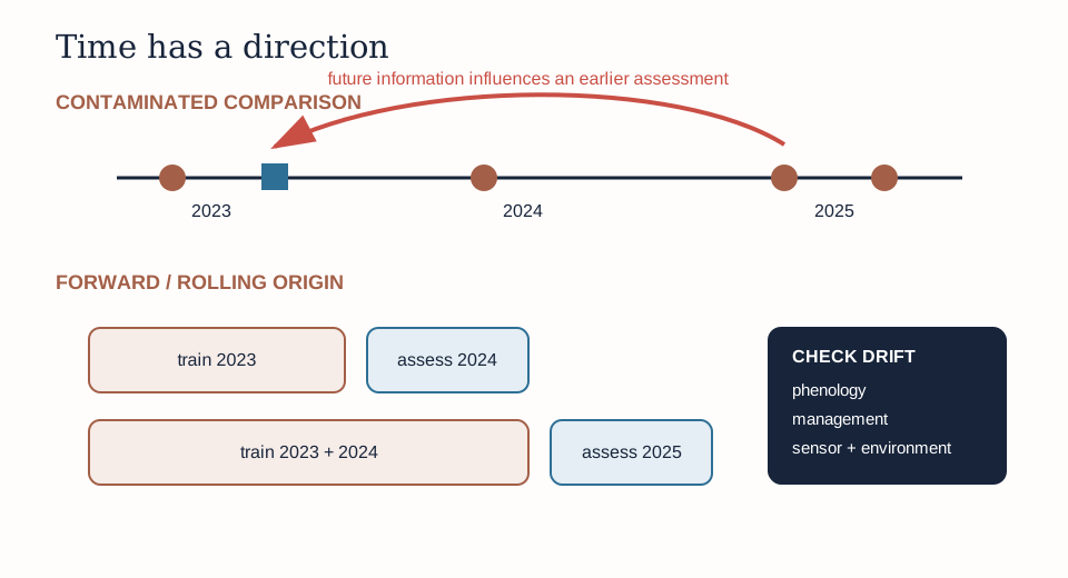
The upper timeline shows why a random split may look independent in row identity yet violate deployment time. The lower design expands the historical evidence only after a period has been assessed. This is a simulation of how information would have accumulated.

The drift box is not decoration. A lower future score can reflect several changing systems. Diagnose before attributing the change to “model decay.”

5. Four kinds of drift a Remote Sensing Scientist must separate

Phenology drift

Vegetation state changes with season, growing degree days, flooding and acquisition date. A model trained on peak-season canopy can fail earlier or later in the phenological cycle. Check day-of-year, field–image gap, stage indicators and target distributions. Do not repair a seasonal mismatch with a model parameter alone.

Management change

Grazing, mowing, restoration or altered hydrology can change the target relationship. A predictor that represented height under one management regime may behave differently after intervention. Management labels must be available at prediction time and measured consistently; post-outcome knowledge creates leakage.

Sensor or processing drift

Sensor calibration, platform, atmospheric correction, UAV camera, flight settings, mosaic pipeline or product baseline can change. A stable ecosystem can still produce a shifted feature distribution. Record sensor and processing versions so a future error increase can be traced.

Environmental drift

Weather, salinity, inundation, drought or disturbance can move observations into predictor and target conditions absent from development. This is not necessarily a technical defect. It can be a domain-of-applicability problem requiring new evidence, an updated model or a restriction on use.

Drift in predictors is not proof that predictive performance changed; target evidence is needed to measure error. Conversely, stable marginal predictor distributions do not prove the conditional relationship is stable.

6. Worked example — create forward year folds

Predict before running

The years are 2023, 2024 and 2025. Predict the training and assessment years in each fold. Will 2025 ever help predict 2024? How many assessment years exist? Write the answer before running.

import pandas as pd

data = pd.read_csv("data/structured_validation_data.csv")
data = data.sort_values(["observation_date", "observation_id"])
years = sorted(data["year"].unique())
fold_rows = []

for fold, test_year in enumerate(years[1:], start=1):
    train_years = years[:fold]
    train_index = data.index[data["year"].isin(train_years)]
    test_index = data.index[data["year"] == test_year]
    assert data.loc[train_index, "year"].max() < test_year
    fold_rows.append({"fold": fold, "train_years": train_years,
                      "test_year": test_year,
                      "n_train": len(train_index), "n_test": len(test_index)})

print(pd.DataFrame(fold_rows))

Code walkthrough

1. pandas loads the synthetic fixture.
2. Sorting by date and stable ID makes temporal order explicit and deterministic.
3. Unique years are sorted from earliest to latest.
4. fold_rows will preserve the design before any model is fitted.
5. The loop skips the first year because no earlier year is available for training.
6. test_year is the next destination in time.
7. train_years contains only years earlier than the current assessment year.
8. Indices are selected by the declared year rule rather than shuffled.
9. The assertion proves that the latest training year precedes the assessment year.
10. The registry records fold, temporal support and counts.
11. The printed table should show 2023 → 2024 and 2023–2024 → 2025.

The assertion checks target-row chronology. You must separately audit when each predictor and preprocessing statistic became available.

Diagnostic check

For every feature, add available_timestamp, source_acquisition_start, source_acquisition_end and processing_version to a provenance audit. Confirm that available_timestamp is at or before the prediction cut-off. If a 2024 composite uses an image from 2025, the row year alone cannot detect the leak.

7. Compare random and temporal holdout without changing the model

Use the fixed Chapter 2 feature order and untuned XGBoost configuration. Compare:

• a random holdout containing observations from all years;
• a chronological holdout that trains on 2023–2024 and assesses 2025.

For both designs, fit the mean baseline on training targets only. Save row-level predictions. Calculate MAE, RMSE, signed bias and baseline skill. Then stratify residuals by site, block, target range and acquisition date.

If chronological error is larger, investigate:

1. whether 2025 target values extend beyond the earlier range;
2. whether feature distributions shift;
3. whether the relationship between predictors and target changes;
4. whether repeated locations make the temporal task easier than a new-location future task;
5. whether sample counts or missingness differ.

Do not tune on the 2025 error. In this lesson, 2025 is assessment evidence for the fixed candidate. Chapter 4 will introduce controlled selection inside development data. If you respond to the 2025 result by altering parameters, that year becomes model-selection evidence and needs a new independent future assessment.

Check your understandingChronological error rises in 2025. What does that prove?

Choose one answer

Transfer weakened in the represented future assessment, but the drift mechanism still needs diagnosisThe sensor alone caused the failureThe model must be tuned on 2025 immediately

Check answer

8. Spatiotemporal validation — name both axes

Create a two-axis claim matrix:

Space	Time	Example destination	Relevant separation
known	represented	another plot in monitored sites and seasons	group repeated sources; row split may be possible
new	represented	unvisited site in similar campaign period	hold out site
known	future	next year at monitored sites	past → future, repeated locations allowed by claim
new	future	unvisited site next year	site and time separation

The last cell is often the real monitoring ambition and the hardest to evaluate. A simple approach may hold out one site and a later year simultaneously, leaving only earlier observations from other sites for training. With few sites and years, the evidence becomes sparse. That limitation should be visible rather than concealed by reverting to random folds.

A complete spatiotemporal registry includes outer fold, held-out site, held-out period, prediction cut-off, training sites, training periods, excluded buffers and the exact IDs used. Examine whether every fold retains enough environmental and target support to fit the model.

9. Model clinic — four temporal leaks that survive a clean row split

Full-period normalisation

Scaling or imputation is fitted using all years before splitting. Future distribution information enters the historical model. Place the transformation inside a fold-local pipeline or explicitly fit on the historical partition.

Retrospective composites

A “2024” feature summarises a window that ends in 2025. Rename the feature with its true support and exclude it from a 2024 prediction.

Intervention labels

A management outcome recorded after the target date is used as a predictor. Check inference-time availability, not merely column completeness.

Repeated model decisions on the latest year

The team repeatedly changes the feature set after viewing 2025 performance. The year becomes validation evidence. Preserve the history, freeze the procedure and collect later independent evidence before a final future claim.

10. Guided practice — build the temporal evidence ledger

1. Add ## Lesson 3.11 — temporal validation to the cumulative notebook.
2. Parse observation_date and verify year consistency.
3. Create a random comparison split and the two rolling-origin folds.
4. Save temporal_fold_registry.csv with observation ID, fold, role, cut-off, year, site and block.
5. Assert that every training date precedes each fold’s assessment period.
6. Complete a predictor-availability table. Mark the fixture’s dates and coordinates as synthetic.
7. Fit the fold-local baseline and fixed candidate.
8. Save predictions with design, fold and time metadata.
9. Plot fold metrics individually and create a residual-by-year plot.
10. Compare predictor ranges and target ranges between historical and future partitions.
11. Write one paragraph each on phenology, management, sensor and environmental drift. State which can be tested with the fixture and which require external metadata.
12. Draft a 2026 monitoring protocol without inventing 2026 performance.

11. Independent challenge — design a future and new-site assessment

The Academy project must eventually support predictions at a new site in a later season. Design a spatiotemporal outer validation using the available four sites and three years.

Specify:

• the exact outer assessment unit;
• whether each fold withholds one site-year combination or a whole future site period;
• how earlier years and other sites enter development;
• how repeated blocks are handled;
• what minimum data requirement could make a fold infeasible;
• how preprocessing and feature construction obey the cut-off;
• which metric distribution and drift tables will be reported;
• why this exercise still cannot prove transfer beyond the synthetic domain.

Include a diagram or table of at least two folds. Do not choose fold definitions after fitting.

12. Common mistakes

Shuffling before a future prediction task

Why: random splitting is familiar and balanced. Recognition: later dates occur in training for earlier assessment rows. Fix: define and assert a cut-off. Consequence: reported performance benefits from unavailable future evidence.

Calling leave-year-out forecasting

Why: whole years are separated. Recognition: some folds train on later years and assess earlier years. Fix: use rolling-origin or a chronological holdout for directional claims. Consequence: the evidence does not simulate deployment.

Sorting rows but fitting preprocessing globally

Why: chronology appears solved by index order. Recognition: imputer, scaler, composite or feature selector saw all periods. Fix: fit transformations inside each fold’s historical training partition. Consequence: future distribution information leaks backward.

Treating drift as one phenomenon

Why: every future error increase is called concept drift. Recognition: sensor version, phenology, management and environmental change are not separately inspected. Fix: maintain a drift register with mechanisms and evidence. Consequence: the response may address the wrong system.

Using time alone for a new-site claim

Why: the latest year feels independent. Recognition: assessment blocks have earlier observations from the same sites in training. Fix: separate both site and time when the destination is new in both. Consequence: spatial familiarity inflates the future-site estimate.

Averaging two temporal folds as precise evidence

Why: cross-validation produces a mean. Recognition: only 2024 and 2025 are assessment periods. Fix: show individual folds and state the small temporal sample. Consequence: two designed years are presented as a stable long-term forecast estimate.

13. Scientific interpretation

A weaker chronological score indicates that the candidate is less accurate under the represented future shift than under the random mixture. It does not by itself identify drift type. Use feature, target, residual and metadata comparisons to develop hypotheses.

A stable score does not guarantee the relationship will remain stable in 2026. The evaluation covers only the designed 2024 and 2025 transitions. Operational monitoring needs target collection, drift triggers and a policy for review.

When the spatiotemporal design becomes too data-poor, the honest result is that the claim is not yet estimable with adequate precision. Collecting another site or season can improve scientific evidence more than another algorithm.

14. Submission

Submit:

• the executed temporal and spatiotemporal notebook checkpoint;
• temporal_fold_registry.csv and temporal_validation_predictions.csv;
• temporal_validation_report.md with random versus chronological metrics, fold values and drift diagnostics;
• one screenshot of the direction-respecting fold diagram or result plot;
• a 350–500 word future-deployment interpretation;
• the proposed 2026 monitoring protocol and its evidence limits.

Portfolio artifact

Structured Validation Design — Part 3: Temporal Transfer and Drift Report

This artifact demonstrates that your model-development evidence respects time, records predictor availability and distinguishes several mechanisms that can weaken future transfer.

15. Reflection

1. Which information in your workflow has a time of availability distinct from its nominal observation year?
2. When is leave-year-out scientifically useful but not a forecasting design?
3. What spatial familiarity remains in a known-site future holdout?
4. Which drift mechanism would require new metadata to diagnose?
5. At what point does repeated use of the latest year convert it into development data?

Check your understandingThe team changes features after viewing 2025 performance. What role does 2025 now have?

Choose one answer

Validation/development evidenceUntouched final-test evidenceNo role because it is a year

Check answer

16. Core references and advanced reading

Core references

• scikit-learn 1.9 — cross-validation for time-series data
• scikit-learn 1.9 — TimeSeriesSplit
• Roberts et al. (2017) — temporal and spatial structure in cross-validation

Optional advanced reading

• scikit-learn common pitfalls — training-only preprocessing
• The Turing Way — reproducible research and provenance

Tested software versions

Python 3.12.13; JupyterLab 4 / Notebook 7; NumPy 2.4.2; pandas 2.2.3; scikit-learn 1.9.0; XGBoost 3.3.0. Verify splitter assumptions for irregular ecological observations and save custom fold registries when a generic time-series iterator cannot encode site, block and availability constraints.