Monitoring Through Repeated Predictions

1. Problem — two prediction maps are not automatically an observation of change

Learning outcome

By the end of this lesson, you will be able to design a repeated-prediction monitoring run; keep target, predictor and grid semantics comparable through time; distinguish data drift, covariate shift, concept drift and observed ecological change; calculate transparent review indicators; define fail-closed release and escalation gates; and interpret differences between predicted maps without claiming that the model directly observed ecological change.

• Lesson type: Repeated Prediction and Drift Laboratory
• Estimated time: 250–350 minutes
• Prerequisites: Lessons 3.11, 3.19, 3.21 and 3.23–3.28; Module 2 time-series, QA and raster delivery skills
• Portfolio outputs: MONITORING_RUNBOOK.md, monitoring run registry, drift dashboard specification, review-trigger tests and the Lesson 3.29 notebook checkpoint

Why this matters

Environmental monitoring is not created by rerunning a model annually. A different sensor baseline, cloud distribution, acquisition date, predictor range or field relationship can change predictions even when vegetation does not change. Conversely, real ecological change can occur while a model remains insensitive to it.

Repeated maps become credible monitoring evidence only when input comparability, model applicability, uncertainty, reference checks and review rules are maintained over time. A system must be able to say “do not compare,” “review this region” or “collect new field evidence,” rather than forcing every run into a green operational status.

Core lesson: predicted change is a model comparison conditioned on stable measurement and model assumptions; it is not direct proof of ecological change.

Mental model

new imagery → acquisition QA → frozen predictors → schema/domain gates
                                                      ↓
                     model version → prediction + uncertainty + applicability
                                                      ↓
        comparable prior run → difference evidence → review/field verification
                                                      ↓
                        release · investigate · withhold · retrain

Each run adds evidence to a monitoring history. It should never rewrite earlier results silently.

2. Scientific context — annual coastal-meadow predictions

Imagine that the group produces a vegetation prediction package each summer. The decision audience wants to know where conditions may have changed enough to justify field review. The model was validated on represented sites and years, but the next season has different rainfall, acquisition timing and cloud availability.

The operational question is not “Did the map colour change?” It is:

Under a stable prediction contract and after input, applicability and uncertainty checks, where did the fixed model produce a difference large enough to require scientific review?

This wording keeps prediction separate from observation. Field surveys, independent imagery and ecological context are required before attributing the difference to management, disturbance or climate.

The supplied monitoring registry is synthetic. Its drift values and release states exercise QA logic; they cannot establish real trends in Baltic coastal meadows.

3. Concept — four changes that must not be confused

Data-quality change

The measurement process changes: more cloud, haze, striping, geolocation error, different missingness or an altered processing baseline. The affected inputs may be less reliable even if their statistical distribution looks familiar.

Covariate shift or predictor drift

The distribution of model inputs changes. NDVI values may extend beyond the training range, predictor correlations may change, or more cells may fall outside the Domain of Applicability. The relationship between predictors and target might remain stable, but the model is being used on less represented inputs.

Concept drift

The relationship between predictors and target changes. The same spectral/structural values may correspond to different vegetation conditions because phenology, species composition, management or sensor relationships changed. Predictor monitoring alone cannot prove or exclude concept drift; new paired reference observations are needed.

Ecological change

The environmental quantity itself changes. This can be the monitoring objective, but a predicted difference remains mediated by the model. Independent evidence and uncertainty are needed to interpret whether the difference is plausible, meaningful and attributable.

These categories can occur together. A drought year can produce true ecological change, predictor shift and a changed predictor–target relationship.

Check your understandingCan predictor distributions alone establish concept drift?

Choose one answer

No; new paired target evidence is needed to evaluate a changed predictor–target relationshipYes; any covariate shift is concept driftYes; a large pixel count proves it

Check answer

4. Visual explanation

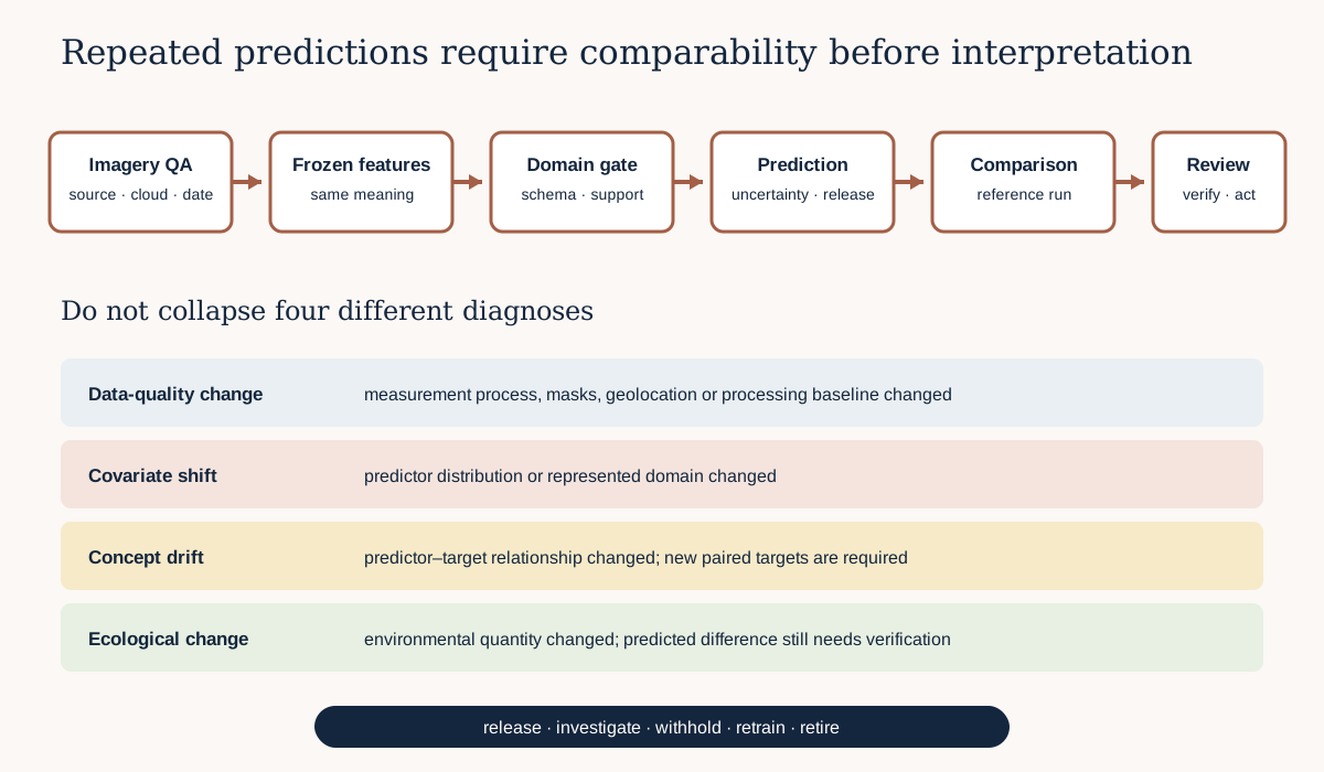
The diagram places review before ecological interpretation. Automation can flag evidence; it cannot decide causation.

5. Freeze what comparability requires

Before scheduling the first repeat, record a monitoring baseline:

• target definition, unit, spatial and temporal support;
• prediction grid, region and valid-population mask;
• source collection, processing baseline and band scaling;
• acquisition window and phenological selection rule;
• cloud/shadow/snow and quality masks;
• composite and gap-filling procedure;
• ordered feature schema and transformations;
• model, uncertainty, applicability and release-policy versions;
• reference run ID and checksum;
• expected QA ranges and review thresholds.

“Use the same month” is insufficient when growing seasons shift. Prefer a scientifically justified phenological rule and record the actual acquisitions used. If the rule cannot be satisfied in a cloudy year, the run should declare limited comparability.

Never overwrite an old predictor or prediction with a new processing baseline. Version the rerun. If a historical series is reprocessed for consistency, retain both lineages and explain why cross-version comparisons changed.

6. Worked example — one fail-closed monitoring gate

monitoring_gate = {
    "schema_match": True,
    "sensor_qa_pass": True,
    "comparable_temporal_support": True,
    "outside_applicability_fraction": 0.08,
    "maximum_outside_fraction": 0.10,
    "coverage_recently_verified": True,
}
release = (
    monitoring_gate["schema_match"]
    and monitoring_gate["sensor_qa_pass"]
    and monitoring_gate["comparable_temporal_support"]
    and monitoring_gate["outside_applicability_fraction"]
        <= monitoring_gate["maximum_outside_fraction"]
    and monitoring_gate["coverage_recently_verified"]
)
print("release" if release else "review")

Predict before running

1. What state will be printed?
2. What happens if the outside fraction becomes 0.14?
3. Does release mean ecological change is confirmed?
4. Why is recent coverage evidence included rather than model age alone?

Run the cell. It prints release. Change only the outside fraction to 0.14; it prints review. This gate is illustrative. A real threshold must be predeclared from decision consequences and monitored evidence, not copied from the lesson.

Code walkthrough

1. The dictionary preserves each condition separately.
2. Schema match checks the prediction-time feature contract.
3. Sensor QA blocks known acquisition or processing failures.
4. Temporal support protects phenological comparability.
5. Outside-applicability fraction summarizes one domain warning across the valid region.
6. The maximum is a governed threshold, not a statistical truth.
7. Recent coverage verification asks whether the interval procedure remains empirically credible on new reference data.
8. The Boolean conjunction is fail-closed: every condition must pass.
9. The output says whether to release the model product, not what happened ecologically.

7. Build run-level and cell-level evidence

Run-level QA determines whether the product can be compared at all. Record source scenes, QA fractions, temporal distance, schema identity, model version, spatial grid, valid area, applicability fractions, interval-width distribution, reference counts and task status.

Cell-level evidence qualifies local interpretation. Preserve prediction, interval bounds, applicability, input validity and release state from Lesson 3.25. Add difference from the selected reference run and, where mathematically appropriate, an uncertainty-aware change flag.

Do not subtract classification codes as though their numeric difference had magnitude. For a probability model, compare calibrated probabilities with consistent class meaning. For a regression model, subtract values only when units, grid, support and target meaning match.

If two prediction intervals overlap, that does not automatically prove “no change.” If they do not overlap, that does not automatically prove change either, especially when interval dependence across time is ignored. Define a change assessment procedure appropriate to the model and repeated measurement design; otherwise present the difference as a review indicator.

Check your understandingTwo comparable prediction maps differ by 12 target units. What has been established?

Choose one answer

The fixed model produced a difference that requires uncertainty and independent ecological reviewEcological decline is provenThe sensor directly measured the target change

Check answer

8. Monitor predictor drift with reference distributions

A useful drift dashboard can report:

• missing or masked fraction by predictor;
• median, interquartile range and robust quantiles;
• fraction outside training min/max;
• multivariate applicability state;
• categorical frequency changes;
• spatial concentration of out-of-domain cells;
• change in predictor correlations;
• acquisition date and quality distribution;
• drift by habitat stratum or management region.

Do not rely on one universal threshold. A small shift in a sensitive red-edge feature may matter more than a larger shift in a stable topographic feature. A population-level histogram may hide a severe regional shift. Link each indicator to measurement meaning and a response.

Formal tests such as Kolmogorov–Smirnov statistics, population stability indices or divergence measures can support screening, but huge raster sample sizes make tiny differences statistically significant. Operational importance should use effect size, spatial pattern and model sensitivity, not p-values alone.

9. Detect concept drift through new labels

Without new target observations, you can monitor inputs and model outputs but cannot directly establish whether the predictor–target relationship changed. Plan a reference programme:

• stable sentinel field plots for continuity;
• rotating probabilistic samples for spatial coverage;
• targeted samples in high-uncertainty and out-of-domain areas;
• independent quality control and preserved observation protocols;
• enough sites and times to assess transfer rather than pixel count;
• protected evaluation before retraining.

Compare new observed targets with frozen-model predictions. Track bias, MAE or classification/probability metrics by site, season and relevant subgroup. If performance degrades, diagnose measurement changes, sampling changes and domain shift before declaring concept drift.

Do not immediately train on every new label. First preserve it as monitoring evidence for the current model. A governance rule should decide which portion can later enter development and which remains protected for the next model version.

10. Define review, retraining and retirement triggers

A trigger connects evidence to an action. Examples include:

• stop run: feature schema mismatch, failed grid check, missing source identity;
• withhold region: outside applicability or invalid input;
• manual review: unusual cloud fraction, temporal mismatch, wide intervals, clustered drift;
• field verification: large supported differences in management-relevant regions;
• recalibrate: interval coverage or probability calibration degrades while ranking remains useful;
• retrain candidate: protected predictive performance falls below the declared floor;
• retire model: target definition, sensor or decision use changes beyond the model card.

Every trigger needs a threshold/rule, evidence window, owner, response time, allowed override, override record and closure criterion. An alert without an operator and response is only noise.

Check your understandingA drift alert has no owner or response procedure. What is its operational value?

Choose one answer

Incomplete; a trigger needs accountable action and closureComplete because dashboards are self-interpretingIt should retrain automatically

Check answer

Retraining is a new model-development cycle. It must preserve versioned data, folds, baseline comparison, protected assessment, model card and parallel comparison with the incumbent. Newer is not automatically better.

11. Diagnostic check — examine a synthetic run history

Open monitoring_runs_fixture.csv and answer:

1. Which runs are comparable to the reference and why?
2. Which run fails before prediction because of schema or sensor QA?
3. Where does outside applicability exceed the frozen limit?
4. Which run lacks recent labelled coverage evidence?
5. Does any row prove ecological change?

Recompute the proposed state from the component indicators. Assert that the computed state equals the recorded state. Then alter one value at a time to test boundary behaviour exactly at and immediately above the threshold.

Finally, map the hypothetical outside-domain fraction by region. A national fraction below threshold can conceal a local region entirely outside support.

12. Common mistakes

Calling a prediction difference observed change

Why beginners make it: subtraction produces a precise number. Recognition: the interpretation omits model, uncertainty and reference evidence. Fix: call it a modelled difference or review indicator until independently supported.

Reusing a fixed calendar window blindly

Why: dates are easy to automate. Recognition: phenological stage differs across years. Fix: use and audit a justified temporal-support rule; withhold incomparable runs.

Monitoring only model outputs

Why: one prediction histogram is convenient. Recognition: source, masks and predictors have no dashboard. Fix: monitor the measurement chain before the output.

Equating covariate drift with concept drift

Why: both can reduce performance. Recognition: the report claims relationship change without new labels. Fix: reserve concept-drift diagnosis for evidence involving new targets.

Retraining on the monitoring test

Why: new labels are valuable. Recognition: the same observations trigger, tune and evaluate the replacement. Fix: establish development and protected partitions before model updates.

Allowing alerts without actions

Why: dashboards appear operational. Recognition: no owner, response or closure record. Fix: turn each indicator into a runbook step or remove it.

13. Guided practice — write the monitoring runbook

1. Copy MONITORING_RUNBOOK_TEMPLATE.md.
2. Name the monitored target and supported decision.
3. Freeze the reference product and comparison grid.
4. Record imagery, masks, temporal rule and predictor schema.
5. List run-level QA indicators and thresholds.
6. List cell/region release states and reason codes.
7. Define new-reference sampling and evaluation cadence.
8. Separate data-quality, covariate and concept-drift checks.
9. Define release, review, withhold, retrain and retire actions.
10. Assign an owner, response time and closure record.
11. Test three failing synthetic runs.
12. Add an accessible text summary for users who cannot inspect a map.

Your first runbook may state that some thresholds are provisional. Record how they will be calibrated and who approves them.

14. Independent challenge — investigate an apparent decline

A new annual prediction is 12 target units lower across one managed region. Create a structured investigation plan covering:

• grid and model-version equality;
• source processing baseline and acquisition dates;
• cloud/shadow and valid-area differences;
• univariate and multivariate predictor drift;
• interval width and applicability;
• spatial pattern and boundary effects;
• independent imagery and field evidence;
• alternative ecological and measurement explanations;
• communication before and after verification.

Write two summaries: one for the scientific team and one for a management audience. Neither may call the result a confirmed vegetation decline without new evidence.

15. Scientific interpretation

A stable operational pipeline can produce comparable model outputs, but it cannot make a model an observing instrument independent of its inputs and training relationship. The safest monitoring language distinguishes the EO measurement, modelled quantity, predicted difference, uncertainty, support and follow-up observation.

An increase in out-of-domain area is itself operationally useful: it says where the existing evidence base no longer resembles current inputs. It is not proof of degradation. A failed coverage audit is also useful because it prevents narrow but unreliable intervals from supporting decisions.

16. Submission

Submit:

• MONITORING_RUNBOOK.md with baseline, cadence, indicators, triggers and owners;
• completed synthetic run registry with reproduced release states;
• a drift-dashboard specification with accessible textual output;
• the apparent-decline investigation plan;
• a version/update policy separating monitoring labels from retraining data;
• the Lesson 3.29 notebook checkpoint;
• a 350–500 word interpretation distinguishing predicted difference, predictor drift, concept drift and ecological change.

Do not submit a time-series animation without run identities, QA and interpretation limits.

17. Portfolio artifact

Artifact 29 — Monitoring Runbook

This artifact turns a one-off prediction pipeline into a governed repeated process. It shows how you will preserve comparability, diagnose drift, collect new evidence and stop unsupported ecological claims before release.

18. Reflection

1. Which kinds of drift can be monitored without new target observations?
2. Why can a below-threshold national drift fraction still require regional review?
3. What evidence distinguishes concept drift from measurement failure?
4. When should an incumbent model be retired rather than retrained?
5. How would you communicate a large but uncertain predicted difference?

19. Core references

• Google Machine Learning — production ML systems and data dependencies
• scikit-learn common pitfalls and recommended practices
• OGC Cloud Optimized GeoTIFF standard

Further advanced reading

• Gama et al. (2014), a survey on concept drift adaptation
• Rabanser, Günnemann and Lipton (2019), failing loudly
• The Turing Way — research data management

20. Tested software versions

The monitoring-gate exercises target Python 3.12.13, NumPy 2.4.2 and pandas 2.2.3. Thresholds and synthetic registry outcomes are instructional, not validated operating limits. An actual system must record sensor collection versions, model packages, spatial libraries and the dated evidence used to approve every trigger.