What Is a Raster Really?

1. Begin with a question an array cannot answer

Learning outcome

By the end of this lesson, you will be able to explain how a numerical two-dimensional array becomes a geospatial raster. You will identify rows, columns, cells, bands, shape, data type, CRS, affine transform, resolution, bounds, extent, NoData, mask and spatial support, then create a defensible raster metadata record for the Module 2 portfolio.

Prerequisites: Module 1's two-dimensional NumPy bridge, Lesson 2.2 on coordinate reference systems and Lesson 2.3 on spatial support. Allow 75–90 minutes. This is a concept and visual lab; no previous Rasterio experience is assumed.

Why this matters

A raster can look like a photograph, a heat map or a coloured classification. That appearance is useful for inspection, but it can hide the data model. Two files can draw in the same place while using different grids. Two arrays can have the same shape while describing different countries. A black cell may mean water, zero reflectance, a class code, masked support or a display choice.

Professional raster work begins by asking four questions:

1. What physical or classified quantity does each stored value represent?
2. Which ground footprint belongs to row r, column c?
3. Which cells are valid for this analysis?
4. Which metadata and provenance support those answers?

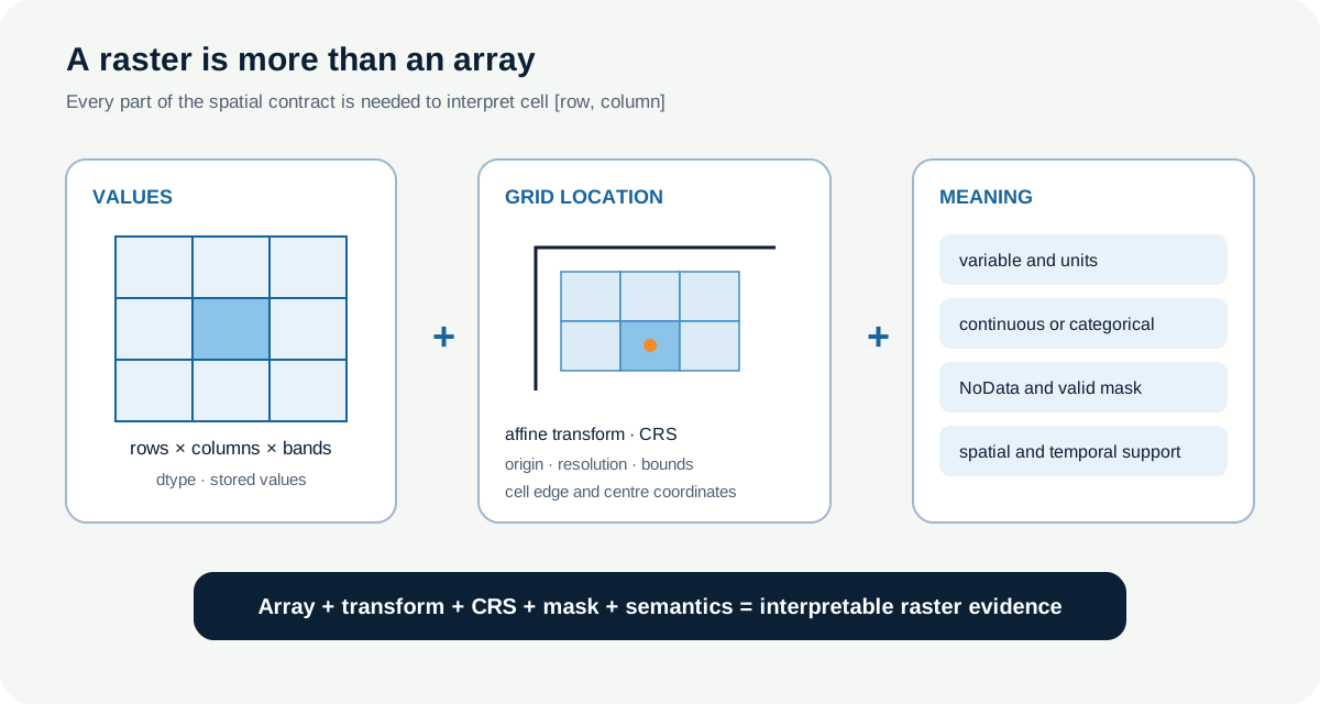
Primary raster principle: A raster is values + grid structure + spatial reference + measurement semantics. A visually convincing raster can still be scientifically wrong.

Scientific context

The Baltic coastal-meadow team is preparing to combine UAV bands, a habitat classification and an elevation surface. The Academy training pack is entirely synthetic; it contains no unpublished imagery or published field coordinates. Its purpose is to make grid decisions observable before governed data are used.

The reference file, aligned_continuous.tif, stores a small continuous surface. Its values resemble a unitless fraction only for teaching. You must not call them measured reflectance. The class raster stores integer habitat codes, but those codes have meaning only because the metadata define them as categories.

Learner action

Create 01_raster_inventory.ipynb inside a new raster_science/ folder. Add the heading ## Lesson 2.11 — What is a raster really?. Beneath it, write what you believe an image pixel represents. Leave the sentence unchanged until the reflection.

2. A two-dimensional array has positions, not Earth locations

Consider this NumPy array:

import numpy as np

grid = np.array([
    [1, 2, 3],
    [4, 5, 6],
])

print(grid.shape)
print(grid[0, 0])

The array has two rows and three columns. grid[0, 0] returns the first stored value. The array can answer questions about index position and numerical value. It cannot answer:

• where the first cell lies on Earth;
• how wide or tall the cell is;
• whether rows advance north or south;
• which coordinate reference system applies;
• what the value 1 measures;
• whether 0, -9999 or NaN would be valid;
• when or how the value was observed.

These are not optional details added after analysis. They determine whether the values can support spatial reasoning.

Check your understandingA 2 × 3 NumPy array contains six values. Which question can it not answer by itself?

Choose one answer

Where cell [0, 0] lies on Earth and what physical quantity it representsHow many rows and columns it hasWhich value is stored at [0, 0]

Check answer

3. The grid model connects indices to cells

A regular raster organises values by row and column. In common north-up rasters, row zero is at the top and row numbers increase downward. Column zero is at the left and column numbers increase to the right. This convention differs from a graph whose vertical coordinate increases upward, so make it explicit.

The array shape is usually reported as (height, width) or (rows, columns). A single-band 12 × 12 raster contains 144 cell positions. A multiband array may be represented in memory as (bands, rows, columns), but software conventions must be checked rather than assumed.

A pixel in this chapter means a grid cell. The cell is an area with edges and a centre. The value stored for that cell can represent a sampled, integrated, estimated or classified quantity. Pixel and measurement are not synonyms:

• the cell is the spatial container;
• the value is the stored representation;
• the measurement semantics explain how that value relates to the phenomenon.

One cell is not automatically an independent observation. Neighbouring cells may share sensor response, processing influence, interpolation or ecological processes.

4. Bands share a grid but represent different variables

A single-band raster stores one value layer: elevation, temperature, NDVI or habitat class. A multiband raster stores several band arrays under one dataset. A coherent stack requires every band to share the dataset grid, dimensions and spatial reference. Band meaning, units, wavelength or class legend remain separate metadata.

Examples for the Academy pathway include:

Band or layer	Semantic type	Value meaning
Red	continuous	calibrated or otherwise documented red-band response
NIR	continuous	near-infrared response under the stated product convention
DSM	continuous	elevation of the represented upper surface
habitat	categorical	integer code linked to an explicit class legend

Do not treat band order as meaning. src.read(1) means the first stored band, not automatically Red. Band descriptions and external product documentation must establish the identity.

5. The affine transform locates the grid

An affine transform connects column and row positions to map coordinates. Conceptually, it tells software:

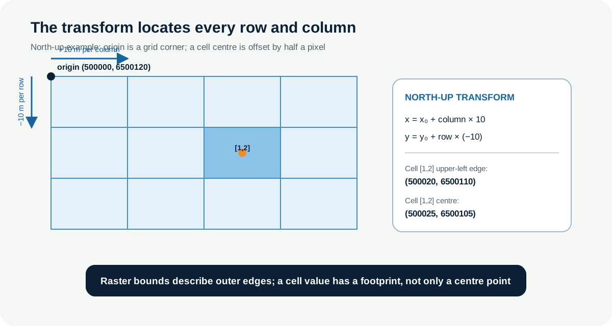
Start at this grid origin. Move by this x step for each column and this y step for each row. Include rotation or shear terms if the grid is not north-up.

For the common north-up case, the transform contains:

• upper-left x coordinate;
• pixel width;
• x contribution from row movement, usually zero;
• upper-left y coordinate;
• y contribution from column movement, usually zero;
• pixel-height step, usually negative because row numbers increase downward.

The origin commonly locates the upper-left outer grid corner, not the centre of the first cell. If the cell is 10 m square, its centre is 5 m east and 5 m south of that corner.

Raster bounds describe the outer grid edges: left, bottom, right, top. They do not imply that every enclosed cell contains valid data. A diagonal study area can occupy only part of a rectangular raster extent.

Check your understandingWhy is the centre of the first 10 m cell offset from the raster origin?

Choose one answer

The origin usually identifies the upper-left grid edge, so the centre is half a cell east and southThe CRS automatically adds five metres to every coordinateRaster rows begin at one rather than zero

Check answer

6. Resolution describes grid spacing, not accuracy

Raster resolution commonly reports the x and y pixel dimensions in CRS units. A 10 m × 10 m cell has a nominal footprint of 100 m² in an appropriate metre-based projected grid.

This number does not prove:

• ten-metre positional accuracy;
• ten-metre effective resolving ability;
• independent information in every cell;
• a ten-metre ecological support;
• that a finer grid came from a finer observation.

Upsampling a 10 m raster to 1 m creates one hundred output cells per original cell area. It does not create one hundred new measurements. Return to Lesson 2.3 whenever pixel size is being used as a quality claim.

7. NoData, masks and NaN describe invalid support differently

Raster workflows need an explicit answer to “Which cells are valid?” Several mechanisms can contribute:

• a declared NoData value, such as -9999 or 255;
• a valid-data mask, where mask values distinguish usable from invalid support;
• NaN in floating-point arrays;
• external quality flags or cloud masks that require a scientific rule.

Zero is not missing by definition. Zero can be valid temperature under a chosen scale, no detected cover, a class label or a real index value. The training file conflicting_nodata.tif deliberately contains a valid zero and explicit -9999 cells. Replacing every zero with missing data would delete evidence.

NoData is also not a physical measurement. Including -9999 in a mean can dominate the result. Use the file mask and documented quality logic, then calculate statistics only over valid cells.

Check your understandingA cell contains zero and the raster declares -9999 as NoData. What is the defensible interpretation?

Choose one answer

Zero remains a potentially valid value unless measurement semantics say otherwiseZero and -9999 are always equivalent missing valuesAll non-positive values should be removed

Check answer

8. Data type constrains storage and interpretation

The raster data type defines how values are encoded. Common examples include:

• uint8: unsigned integers from 0 to 255, often used for class codes or compact display values;
• uint16: a wider unsigned range, often used for scaled sensor values;
• int16: signed integers, allowing negative stored values;
• float32: continuous values with moderate floating-point precision;
• float64: greater precision and twice the storage per value relative to float32.

Data type affects range, precision, file size and the available NoData convention. It does not establish units or semantics. A uint16 value of 5320 could represent a scaled reflectance, elevation offset, quality bit pattern or arbitrary identifier. Scale and offset metadata may be required to recover physical values.

Do not cast types merely to reduce file size. Converting continuous floating values to integers can quantise the result; converting a class raster to floating point does not make its classes continuous.

9. Worked example — reconstruct one cell centre

Predict before running

A grid begins at upper-left corner (500000, 6500120). Each cell is 10 m square. Predict the centre coordinate for row 1, column 2. Remember that row movement is southward.

x_origin, y_origin = 500_000, 6_500_120
pixel_width, pixel_height = 10, -10
row, col = 1, 2

x_centre = x_origin + (col + 0.5) * pixel_width
y_centre = y_origin + (row + 0.5) * pixel_height

print(x_centre, y_centre)

The centre is (500025, 6500105) in the coordinates and units of the raster CRS. The calculation does not identify the CRS, variable, accuracy or valid-data status; those remain parts of the metadata record.

Code walkthrough

1. x_origin and y_origin locate the upper-left grid edge.
2. pixel_width moves east by 10 coordinate units per column.
3. pixel_height is negative because increasing row indices move down a north-up grid.
4. row and col identify the requested array position.
5. Adding 0.5 moves from the cell edge to its centre.
6. The x equation advances two whole columns and half a cell.
7. The y equation advances one whole row and half a cell southward.
8. The printed coordinate becomes meaningful only when attached to the verified CRS.

10. Common mistakes and recovery

Treating a raster as a picture

Why it happens: the first encounter is usually a rendered image. Recognition: interpretation refers to colour but not values, bands, units or masks. Fix: inspect stored values and metadata before choosing a renderer.

Assuming same shape means same place

Why it happens: two arrays can be combined in NumPy. Recognition: cell arithmetic is performed without CRS and transform checks. Fix: treat shape as one field in a complete grid contract.

Assuming smaller pixels are more accurate

Why it happens: finer grids look detailed. Recognition: quality is inferred from cell size alone. Fix: report resolution separately from positional, radiometric and thematic accuracy.

Treating NoData as zero

Why it happens: both may render dark or be used as convenient fill values. Recognition: a zero test replaces the documented mask. Fix: inspect NoData, masks, quality flags and valid zero behaviour separately.

Forgetting that a cell has area

Why it happens: extraction APIs return one value at a coordinate. Recognition: a centre value is presented as the full support of a field observation. Fix: document cell footprint and compare it with the measurement support.

11. Guided practice — build a raster anatomy record

Create a synthetic 4 × 5 array in your notebook. Do not call it observed data. Add a metadata dictionary containing:

1. width and height;
2. band count and band meaning;
3. data type;
4. CRS identifier;
5. upper-left origin;
6. x and y resolution;
7. affine transform coefficients;
8. bounds;
9. NoData and mask rule;
10. continuous or categorical semantics;
11. value units;
12. spatial and temporal support;
13. provenance and synthetic status.

Calculate the centre and outer bounds of cell [0, 0] and one interior cell. Draw the grid and label row direction, column direction, origin, outer bounds and one centre. Then state what still prevents this metadata dictionary from becoming a real remote-sensing observation: acquisition, calibration, sensor response, validation, timing and provenance.

Raster QA check

Open the training-pack manifest.json as text. Locate aligned_continuous.tif and verify that all required fields are present. Compare the transform with the expected 10 m grid and predict the lower-right outer bound from origin, width and height. Do not use a map to answer first.

In QGIS, load the raster only after writing the prediction. Turn on pixel-grid display at a suitable zoom, inspect Layer Properties and use Identify Features on one declared cell. Compare QGIS metadata with the manifest. Visual agreement is supporting evidence, not proof of correct measurement semantics.

12. Independent challenge — diagnose six statements

Classify each statement as supported, unsupported or conditionally supported, and explain why:

1. “Both rasters are 12 × 12, so their cells align.”
2. “The pixel size is 10 m, so positions are accurate to 10 m.”
3. “The value is zero, so the cell is missing.”
4. “The file has EPSG:3301 and a transform, so it is geospatial.”
5. “The habitat raster contains integers, so bilinear interpolation is safe.”
6. “The DSM cell contains elevation, so it represents bare terrain.”

For every unsupported statement, name the missing evidence or the later lesson that will resolve it.

Scientific interpretation

The raster anatomy record can establish how stored positions relate to a declared grid and how values are intended to be interpreted. It cannot validate the truth of the CRS, positional accuracy, calibration, class legend, elevation surface or ecological relevance. Structural completeness is necessary for science, not sufficient for it.

13. Reflection, submission and portfolio artifact

Answer in your private notes:

1. What can a NumPy array answer without geospatial metadata?
2. Why is the affine origin usually not the first cell centre?
3. What is the difference between cell footprint and stored value?
4. Why can extent include invalid cells?
5. Which metadata field most changes how you would analyse a raster?

Submission

• Notebook: 01_raster_inventory.ipynb with the 4 × 5 array, complete metadata dictionary, cell-coordinate calculations and six-statement diagnosis.
• Screenshot: the labelled grid beside the metadata record.
• Written answer: 180–240 words explaining why an array is not yet a geospatial raster and what the completed record still cannot validate.

Portfolio artifact

Artifact 2.11 — Raster anatomy and metadata record

Place the artifact at the beginning of the Raster QA and Harmonisation Pipeline. Every later input must receive the same metadata-first treatment before values are read or transformed.