QGIS for Professional Spatial QA

1. Use visual inspection as evidence, not as a substitute for reproducibility

Learning outcome

By the end of this lesson, you will be able to open a controlled QA project in QGIS; distinguish project CRS, layer CRS and on-the-fly display transformation; inspect source, schema, geometry and attributes; apply diagnostic styling; run validity and join checks through the Processing Toolbox; inspect a raster without treating its appearance as quantitative proof; record anomalies without overwriting source data; and export a clear QA map and observation report that link back to the Python workflow.

Prerequisites: Complete Lessons 2.5–2.9. No previous QGIS experience is required. Install a current supported QGIS release from the official QGIS website before the guided practice. Allow 140–180 minutes.

Why this matters

Code is excellent at repeatable counts, assertions and transformations. A map is excellent at revealing spatial patterns that a summary table can miss: a shifted layer, unexpected striping, an isolated polygon, a point on a disputed boundary, a clipped edge or a symbology rule that hides missing categories.

Neither view is sufficient alone.

• A layer can look aligned because QGIS transforms it for display even though the processing CRS was wrong.
• A polished map can conceal invalid geometry or dropped records.
• A table can pass every programmed check while a layer sits in the wrong coastline or contains a visible digitising artefact.
• A manual correction can fix the display while destroying reproducibility if it is not returned to the scripted workflow.

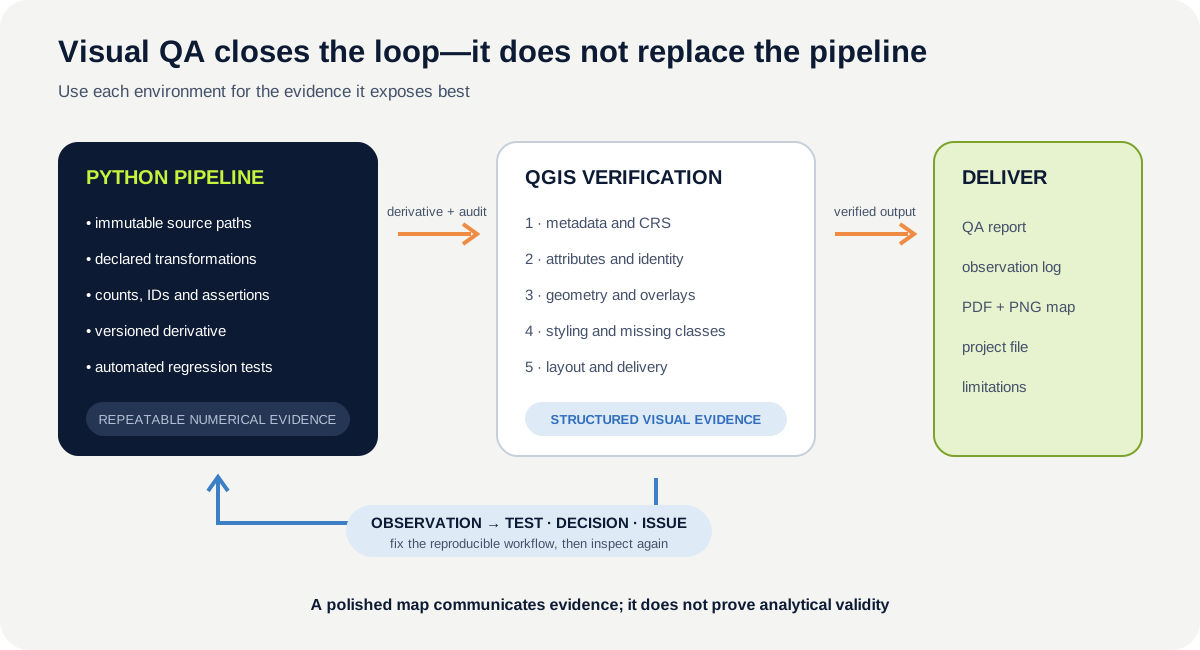
Core QA principle: Python performs reproducible processing. QGIS supports rapid visual verification. Observations found in QGIS become documented tests or decisions in the pipeline.

Scientific context

The coastal-meadow team has produced vector derivatives from Lessons 2.5–2.9. Before beginning raster science, the team needs a visual checkpoint. You will inspect the synthetic training plots, study area, management zones, topology cases and one reviewed derivative.

The training coordinates and classes remain synthetic. A basemap can help detect gross displacement, but it cannot authenticate the invented locations or convert them into published observations.

Learner action

Create a folder named qgis_qa/ inside the Module 2 project. Save a new QGIS project as coastal_meadow_vector_qa.qgz. Copy the downloadable QA checklist and observation-log template into this folder. Do not edit files in data/raw/.

2. Understand the QGIS workspace before clicking

QGIS is a desktop geographic information system. Its interface is organised around several working areas:

• Map canvas: draws the current map view.
• Layers panel: controls layer order, visibility and styling access.
• Browser panel: navigates files, databases and services.
• Data Source Manager: connects to vector, raster, database and web sources.
• Attribute table: displays one record per vector feature and supports selection and filtering.
• Processing Toolbox: runs documented algorithms such as validity checks, fixes, clips and joins.
• Status bar: reports scale, coordinates, rotation and project CRS.
• Print Layout: creates controlled map outputs separate from the analysis canvas.

A project stores display, layer references, styles and layout definitions. It does not automatically copy the underlying data into the .qgz file. Moving a project without its referenced layers can break paths. Use a clear folder structure and relative paths where suitable.

Record the QGIS version in the observation log. Menu wording and algorithms can evolve, so version evidence helps another person reproduce the inspection.

3. Project CRS and layer CRS answer different questions

Every spatial layer should have its own CRS metadata. The project also has a CRS controlling the map canvas. QGIS can transform layers on the fly so data in different CRSs appear together.

This display convenience does not rewrite the source and does not prove that its CRS was assigned correctly.

For each loaded layer:

1. open Layer Properties → Information and record source path, provider, geometry type, extent, feature count and layer CRS;
2. inspect the project CRS shown in the status bar;
3. compare these values with the Python audit;
4. investigate any mismatch before trusting visual alignment.

If a layer with wrongly labelled coordinates happens to draw near another layer, appearance is not evidence. Return to Lesson 2.2: determine the source CRS from provenance, assign only what is known, then transform in the reproducible pipeline.

Check your understandingTwo layers appear aligned in the QGIS canvas. What has this established?

Choose one answer

Only visual agreement under the current project display; layer CRS provenance still requires verificationBoth source files definitely contain correctly assigned CRS metadataQGIS has permanently reprojected both source files

Check answer

4. Build a controlled layer stack

Load data through Layer → Add Layer or the Data Source Manager. For this exercise add:

1. the immutable synthetic study area;
2. management and vegetation zones;
3. synthetic field plots;
4. the topology-case layer;
5. your reviewed derivative from Lesson 2.9.

Rename each layer in the Layers panel with both stage and purpose, for example RAW — topology cases and DERIVED — reviewed analysis zones. A display name does not rename the source file; it helps prevent accidental comparison of the wrong stage.

Arrange polygons below points. Use different outline patterns for source and derivative layers. Keep opacity high enough to inspect boundaries but low enough to compare overlaps. Save style choices in the project, not as undocumented changes to attributes.

Do not add a basemap by habit. It introduces another dataset with its own date, scale, licence and positional limitations. If you use one for broad location QA, record its provider and purpose, and do not present it as validation of ecological boundaries.

5. Diagnostic styling asks a question

Good QA styling makes specific conditions visible:

• categorised colour by qa_case reveals whether every expected class appears;
• a distinct symbol for null or unclassified values prevents them from blending into the background;
• thin source outlines over thick candidate outlines reveal changed boundaries;
• labels using stable IDs connect map features to the decision log;
• rule-based styling can highlight invalid, unresolved or duplicate candidates;
• a visible selection colour helps verify filtered records.

Avoid choosing a visually pleasing classification first. State the question: “Which features changed geometry type?” or “Where do source and reviewed boundaries diverge?” Then style the variable that answers it.

Check the legend. If a category is absent, determine whether no features contain it, the filter excludes it or the style omits it. A map that silently suppresses null values is incomplete QA.

6. Inspect attributes and identity

Open the attribute table for each vector layer. Confirm:

• displayed row count matches the Python audit;
• stable identifiers are present and unique where expected;
• field names and types are plausible;
• null values are visible;
• selected map features correspond to selected table records;
• source and derivative identifiers remain traceable.

Use Select by Expression for diagnostic queries. For example:

"status" = 'needs_authority'

The expression selects records; it does not alter data. Save important expressions in the QA report so another reviewer can repeat them.

The Field Calculator can create or update attributes. Practise only on a copied derivative layer. Create an area_m2_qa field after confirming a metre-based projected CRS, and compare it with Python-calculated area. If the values differ, check CRS, ellipsoid/measurement settings, precision and whether geometry changed. Do not edit the raw source simply to make the numbers agree.

Check your understandingQGIS reveals a suspicious repaired boundary. What is the professional next step?

Choose one answer

Record the affected ID and evidence, correct the governed Python rule if justified, regenerate and inspect againMove the boundary in the only raw file until it looks rightHide the source layer and keep the displayed derivative

Check answer

7. Worked example — define the inspection before opening QGIS

Before running, predict which checks are numerical, which require visual inspection and which require both.

qa_manifest = [
    {"id": "Q01", "check": "CRS and extent agree", "evidence": "both"},
    {"id": "Q02", "check": "row and ID counts agree", "evidence": "numeric"},
    {"id": "Q03", "check": "changed boundaries are explained", "evidence": "both"},
    {"id": "Q04", "check": "null classes are visible", "evidence": "visual"},
    {"id": "Q05", "check": "invalid geometry is reported", "evidence": "numeric"},
    {"id": "Q06", "check": "map labels match IDs", "evidence": "both"},
]

for item in qa_manifest:
    print(f"{item['id']} · {item['evidence']} · {item['check']}")

Code walkthrough

1. qa_manifest is a list of structured checks prepared before visual review.
2. Every check has a stable ID for linking evidence and observations.
3. Q01 requires metadata evidence and a map-based plausibility check.
4. Q02 is primarily a numerical identity test.
5. Q03 connects measured change to visible location and documented reason.
6. Q04 checks whether styling exposes missing categories.
7. Q05 belongs in reproducible geometry diagnostics.
8. Q06 compares label rendering with stable table identity.
9. The loop prints the declared protocol in order.
10. The formatted string keeps check ID, evidence class and instruction together.

Copy the printed manifest into the QGIS QA report. Add columns for result, evidence_file, affected_ids, severity, decision_owner and follow_up.

8. Run geometry validation without accepting automatic fixes

Open Processing → Toolbox and search for Check validity. Use the reviewed derivative as input and keep the algorithm outputs as temporary or explicitly named diagnostic layers. The tool separates valid, invalid and error evidence depending on the selected method and QGIS version.

For each reported issue:

1. record the stable feature ID and error message;
2. zoom to the error location;
3. compare source, repair candidate and reviewed derivative;
4. check whether Python reported the same condition;
5. classify it as confirmed defect, expected structure or unresolved discrepancy.

The Fix geometries algorithm can create another candidate derivative. It is not an instruction to replace the reviewed layer. If you test it, save a new output, compare counts/types/area and return the adopted rule to Python so the production workflow remains reproducible.

9. Verify joins through both map and table

For an attribute join, inspect the key field's nulls and uniqueness before configuring Layer Properties → Joins. A temporary project join changes the displayed layer view, not necessarily the source file. Record the join key, expected cardinality and whether the result must later be materialised by the pipeline.

For a spatial relationship, use the Processing Toolbox's Join attributes by location only as an independent QA comparison. Declare the predicate and expected one-to-many behaviour first. Compare its output with Lesson 2.7:

• input and output row counts;
• unmatched plot IDs;
• repeated plot IDs;
• boundary case TP04;
• outside case TP05.

If QGIS and Python disagree, do not choose the table that looks cleaner. Compare CRS, predicate, boundary semantics, input layer version, selected-feature filters and software versions.

10. Inspect raster layers without analysing them yet

QGIS can display rasters, but Raster Science begins in Lesson 2.11. At this checkpoint, learn only the visual and metadata inspection role.

When a UAV orthomosaic or satellite raster becomes available:

1. inspect Layer Properties → Information for CRS, extent, dimensions, pixel size, bands, data type and NoData;
2. compare those values with the delivery metadata;
3. use the Identify tool on a few declared locations;
4. inspect whether NoData edges, seams, stripes or unexpected values are visible;
5. review the renderer and stretch because display settings can make the same values appear very different;
6. never estimate quantitative validity from colour alone.

Do not resample, reproject or edit the raster during visual QA without creating a named derivative and recording the operation. Later lessons will teach those transformations explicitly.

11. Record anomalies as actionable evidence

An observation such as “the map looks wrong” is not reproducible. Each QA record should include:

• observation ID and timestamp;
• reviewer and QGIS version;
• project CRS and layer source path;
• affected stable feature IDs or map extent;
• check performed and expected result;
• observed result;
• screenshot or exported evidence filename;
• severity: informational, review, blocking;
• proposed action and decision owner;
• final disposition and linked code/test change.

Avoid storing only screenshots. A screenshot cannot be filtered, rerun or reliably linked to features without structured context. Pair it with the observation table.

When QGIS reveals an actual processing defect, update the Python code and its automated checks, regenerate the derivative, then repeat the visual check. Do not repair only the displayed copy.

12. Export a QA map, not a decorative poster

Use Project → New Print Layout to create a controlled review map. Include only elements that support interpretation:

• precise title describing source/derivative and QA purpose;
• map frame at an appropriate scale;
• legend with meaningful layer and class names;
• scale bar when distance interpretation is relevant;
• CRS identifier;
• data-source and derivative-date note;
• author/reviewer and QGIS version in the report metadata;
• annotation or inset for unresolved cases.

A north arrow is useful only when orientation is not already obvious and the chosen map context makes it meaningful. Decorative elements should not displace evidence.

Export both PDF and PNG. Verify the exported files—not only the layout preview—for clipped labels, unreadable text, missing legend classes, incorrect transparency and page size. Record export resolution and filenames.

Check your understandingWhich statement best describes a professional QA map export?

Choose one answer

It communicates source, purpose, CRS, classes and limitations and is reopened after export for verificationIts attractive styling proves the analysis is correctIt needs every decorative map element regardless of purpose

Check answer

13. Common mistakes and recovery

Trusting on-the-fly alignment

Why it happens: layers draw together in the canvas. Recognition: layer and project CRS evidence were never compared. Fix: inspect each layer's source CRS, extent and Python audit; treat display transformation as convenience, not validation.

Editing the only source layer

Why it happens: a geometry can be moved quickly with editing tools. Recognition: no immutable before state or reproducible instruction exists. Fix: cancel or revert, restore the source and create a named derivative through the governed workflow.

Styling away nulls

Why it happens: default categories focus on populated values. Recognition: table null counts exceed visible unclassified symbols. Fix: add an explicit null/unresolved style and report its count.

Accepting Fix geometries as the decision

Why it happens: the algorithm produces a valid output layer. Recognition: changed types and areas were not reviewed. Fix: treat the output as a candidate, compare it with Lesson 2.9 evidence and implement any accepted rule reproducibly.

Exporting without reopening

Why it happens: the layout preview appears correct. Recognition: the delivered PDF has missing fonts, clipped content or an incomplete legend. Fix: open the actual PDF and PNG, inspect at normal size and record the review.

14. Guided practice — complete the vector QA checkpoint

Follow the downloadable checklist in order.

1. create and save the project with a recorded QGIS version;
2. set and record the project CRS;
3. load raw and derivative vector layers from known paths;
4. capture source, provider, CRS, extent, type and count for each layer;
5. apply diagnostic styling for QA cases, nulls and changed boundaries;
6. compare attribute counts and stable IDs with Python;
7. calculate area on a copied derivative and compare selected values;
8. run Check validity and reconcile results with the topology report;
9. reproduce one Lesson 2.7 spatial assignment as an independent check;
10. inspect TP04, TP05, the repair candidate, duplicate geometry and sliver;
11. record every anomaly in the CSV template;
12. export one PDF and one PNG QA map;
13. reopen both exports and complete the delivery checks;
14. add any confirmed discrepancy as a Python test or decision-log update.

Required QA evidence

The report must identify all layer versions and paths, distinguish project and layer CRS, reconcile numerical counts, show diagnostic styling, include validity results, list affected stable IDs and link each observation to a resolution state.

15. Independent challenge — conduct a blind source-versus-derivative review

Hide layer names and ask a colleague—or yourself after a break—to compare source and derivative using only the declared QA protocol. The reviewer must identify:

• where geometry changed;
• which records are unmatched or repeated;
• which feature remains scientifically unresolved;
• whether map styling exposes all statuses;
• whether the exported layout communicates provenance and limitations.

Then reveal the processing stages. Record which changes were detected, missed or incorrectly inferred. Convert one missed condition into an improved Python assertion, QGIS style rule or checklist item.

Scientific interpretation

Visual agreement can support confidence that a derivative occupies the expected region and that known changes are visible. It cannot establish boundary truth, temporal compatibility or ecological validity. QGIS QA becomes scientifically useful when every observation is tied to a source, feature, test and decision—not when the map merely looks convincing.

16. Reflection, submission and portfolio artifact

Answer in your private notes:

1. Why can layers appear aligned when their source CRS handling is wrong?
2. Which checks belong in Python, QGIS or both?
3. Why should a QGIS-discovered repair be returned to the scripted workflow?
4. What can raster display settings hide or exaggerate?
5. What makes a QA map reproducible enough for professional review?

Submission

• Project: coastal_meadow_vector_qa.qgz with portable layer references and diagnostic styles.
• File: qgis_visual_qa_report.pdf, completed observation CSV and exported QA map PNG.
• Screenshot: the QGIS canvas showing source/derivative comparison and at least one selected QA case.
• Written answer: 220–300 words separating reproducible processing evidence, visual evidence and unresolved scientific evidence.

Portfolio artifact

Artifact 2.10 — Professional vector QA map and reconciliation report

This artifact demonstrates that you can connect reproducible Python processing to disciplined desktop GIS review. Add the project, structured observations, final map and feedback-to-code record to the quality-assurance stage of the UAV and Satellite Analysis Pipeline.